If you are getting started in your data science journey and don’t come from a technical background (like me), then you definitely understand the struggle of keeping up with the terminology of data pre-processing.
For the past few months, I’ve tried to really understand all the terms and transformation strategies used by professors, yet I still felt that their description and impact on my models weren’t entirely clear.
This was obviously a concern, considering that Data Scientists spend 60% of the time cleaning and organizing data!

Therefore, I’ve decided to dive deeper into the topic of data pre-processing, outline the basics, and share it with all of you.
This is the FIRST article, so we will only focus on key terms. Make sure to follow me, in order to read the next posts more focused on feature engineering, model selection, etc.
Keep in mind that some of these terms differ depending on the language or platform you are using. But, I hope it gives you a nice overview.
Basics of Data Structure:
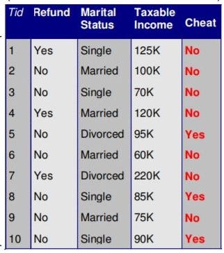
Data objects: an instance or observation containing a set of characteristics. For example, every person (row) on the table.
Attributes: characteristics of an object . Also called features, variables, tuples, or dimensions. For example, the marital status (column) per person (row).
Record: Data that consists of a collection of objects, each of which consists of a fixed set of attributes. For example, the table above. Records aren’t the only type of data set, but the most common, so we will focus on this ones for now.
Vector: a collection of values for an attribute. For example, ‘Single, Married, Divorced’ for Marital Status. All values should be the same data type.
Matrix: in general terms, it is the same as a table but more flexible. The secret is that matrices are all composed of data the same type, and you can apply algebraic functions to them.
Frame: a frame, can be seen as a “snapshot” of a table. Usually used in R, to reduce the size of the table we are working with, or create a new format. We use data frames, instead of matrices or vectors when columns are of different data types (numeric/character/logical etc.).

Types of Records:
- tabular: flat, rows represent instances and columns represent features. Could be like the table above, but also like the table below.
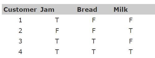
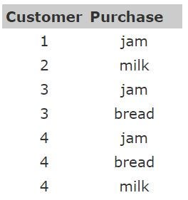
- transactional: rows represent transactions, so if a customer makes multiple purchases, for example, each would be a separate record, with associated items linked by a customer ID.
Basics on Attributes:
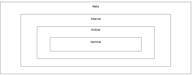
There are four types of data that may be gathered, each one adding more to the next (if gathered correctly). Thus ordinal data is also nominal, and so on. A useful acronym to help remember this is NOIR (French for ‘black’).
Type of Data:
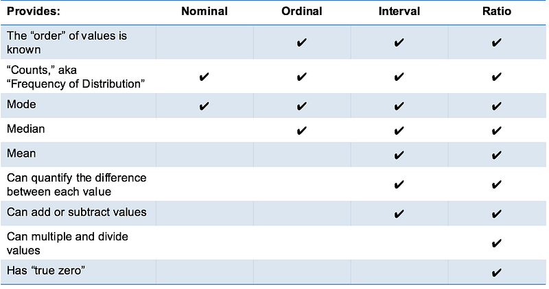
- nominal (qualitative): used to “name,” or label discrete data. (categorical, unordered)

- ordinal(quantitative): provide good information about the order of choices, such as in a customer satisfaction survey. (categorical, ordered)

- interval(quantitative): give us the order of values + the ability to quantify the difference between each one. Usually used with continuous data.
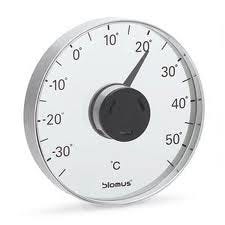
- ratio/scale (quantitative): give us the ultimate–order, interval values, plus the ability to calculate ratios since a “true zero” can be defined.

— — — — Side Note #1:
Interval and ratio data are parametric, used with parametric tools in which distributions are predictable (and often Normal).
Nominal and ordinal data are non-parametric, and do not assume any particular distribution. They are used with non-parametric tools such as the Histogram.
Qualitative data commonly summarized using percentages/proportions, while numeric summarized using average/means.
— — — — end.
Sub-set of Data Types:
- binary/ dichotomous(qualitative): type of categorical data with only two categories. Can describe either nominal or ordinal data. ex. M vs F (or 0 vs 1 when converted in dummy variables)
- discrete(numeric): gaps between possible values. ex. number of students
- continuous(numeric): no gaps between possible values. ex. temperature
Common Types of Values:
- decimal: numeric values to the right of the decimal point, should specify precision and scale (see source: SQL Data Types).
- integer: accepts numeric values with an implied scale of zero. It stores any whole number between 2#k8SjZc9Dxk -31 and ²³¹ -1.
- boolean: accepts the storage of two values: TRUE or FALSE.
- date/time/time stamp: accepts values based on format specified.
- string: basically a “word”, made up of characters. But, sometimes you need to convert an integer into a string in order to treat is as non-numeric.
— — — —Side Note #2:
When the precision provided by decimal (up to 38 digits) is insufficient, use float or real type of values.
- FLOAT[(n)]: used to store single-precision and double-precision floating-point numbers.
- REAL: A single-precision floating-point number.
- DOUBLE [PRECISION]: A double-precision floating-point number.
A single-precision floating-point number is a 32-bit approximation of a real number. The number can be zero or can range from -3.402E+38 to -1.175E-37, or from 1.175E-37 to 3.402E+38. The range of n is 1 to 24. IBM DB2 internally represents the single-precision FLOAT data type as the REAL data type.
A double-precision floating-point number is a 64-bit approximation of a real number. The number can be zero or can range from -1.79769E+308 to -2.225E-307, or from 2.225E-307 to 1.79769E+308. The range of n is 25 to 53. IBM DB2 internally represents the double-precision FLOAT data type as the DOUBLE [PRECISION] data type.
If n is not specified the default value is 53.
— — — — end.
Key Takeaway: You can have, for example, a record with an attribute that is qualitative, categorical, ordinal, continuous, with decimal as a value and that you might need to identify it as real to increase precision. Each of these descriptors will determine how you clean, model and test the data.


