Ready to learn Data Science? Browse courses like Data Science Training and Certification developed by industry thought leaders and Experfy in Harvard Innovation Lab.
Machine learning is the concept of using algorithms to identify patterns and / or make predictions based on an input data set. There are a wide range of algorithms available, each with their own advantages and disadvantages and levels of complexity. These algorithms are readily available and highly accessible through a number of programming tools (R and Python among many many others) with varying levels of coding requirements. They can remove the need for detailed coding instructions tailored specifically to your application and instead use largely generic instructions.
Machine learning differs from classical calculations in that it has the ability to ‘learn’ and make decisions (based on set parameters) as to how it should structure itself in order to achieve an optimal outcome. For example it can access the metrics used to measure the model’s accuracy to change parameters, thus self-optimising.
Machine learning represents the future — or present for some — of advanced analytics. When you or the analysts have completed the data gathering and high level analytics, maybe its time to consider machine learning rather than brute-forcing advanced solutions through tools like Excel. Machine learning provides fast, accurate and flexible solutions which may represent the next step in analytics for your business.
Machine learning can be segmented into supervised and unsupervised algorithms, and then further into the types of outputs they are trying to achieve — classification, regression or clustering. To clarify the differences between these three output types, let us consider a data set based on a group of people’s attributes. Classification may involve trying to label each individual as either ‘short’ or ‘tall’, regression would attempt to predict how tall each person is, and clustering is where there are no height labels and instead the algorithm will cluster people together based on their similar features (e.g. similar weights or shoe sizes which may indicate someone is tall or short).
 Comparison of the three common output types produced through machine learning. Icons made by Freepikfrom www.flaticon.com is licensed by CC 3.0 BY
Random Forest, a supervised learning algorithm, is one of the more simplistic solutions commonly used for classification or regression problems. The algorithm attempts to make a ‘forest’ of decision ‘trees’ which can then be used to collectively predict an outcome. A decision tree is simply the map of the decisions made before reaching an outcome. For example, to the question “Do I need a coffee?”, some of the variables which impact my decision may be “Is the sun still up?”, “Have I already had five coffees?”, “Am I at work?” etc. The decision tree for this critical question is shown below. At each decision, the tree steps to the left if the answer is ‘Yes’ and to the right for ‘No’.
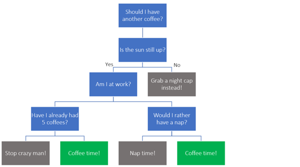
My personal decisioning process for grabbing a coffee. This is a slow decision process without machine learning…
In a Random Forest machine learning scenario, the forest may consist of hundreds of these decision trees which are all based on random sub-sections of the training data set. When the model is provided new data (the test set), each row (observation) is passed through all of the decision trees and each tree provides a suggested classification. The classification provided by the largest number of trees is the one selected and returned by the algorithm. The random nature of data subset selection is one of the features of this algorithm which makes it very robust. When combined with its ease of application, random forest is often one of the first ‘go to’ machine learning algorithms for many data scientists.
The rest of this blog does become slightly more technical to give you a deeper introduction through a worked example. Please don’t stop reading as I hope the rest of the story is still interesting and hopefully helpful to anyone considering learning more about machine learning!
For our example, a dummy data set of house prices was created with five variable columns including number of bedrooms, bathrooms and parking spaces, as well as the block size and build year. The aim of the activity is to build a model to predict the Value of any future houses based on the same variables being available.
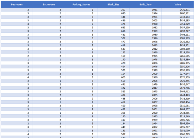
Sample house price data set. 2000 rows of data with 1- 4 bedroom properties, varying numbers of
bathrooms, parking spaces and block sizes and ultimately varying final values.
Building a pricing model is an incredibly open task as it could be approached any way the user sees fit, from completely manual (pen, paper and instinct) to semi-automated modelling in Excel or even artificial intelligence and deep learning / neural networks. The solution we will look at will use a simple binary decision tree generated in R.
Manually preparing a model in this instance wouldn’t be too challenging as there are only five variables. If this example was more typical of a real-world situation, we would be likely to have far more columns which would exponentially increase complexity. A manual model may also become challenging when additional features need to be included in the future. The model would need to be modified and depending on how it was built could require a significant effort. Further, the quality of the model is heavily dependent on the individual or team who prepared it which presents a risk for long term reliability.
The first 1,400 rows of our 2,000 row data-set was split into a ‘training’ set, with the remaining 600 rows separated into our ‘test’ set. The reason this is done is to allow the model access to the first 1,400 rows, enabling it to learn the best predictors of Value. The model is the applied to the test set to predict Values and allow us to check the accuracy. This is done for a variety of reasons however one of these is to reduce the likelihood of ‘over-fitting’ where the model perfectly predicts the outcomes from the training data set but is not general enough to accurately predict new observations.
A binary decision tree was created in R (each decision has two possible outcomes) to provide predicted property Values based on the training data set. Like many algorithms used in R, there are a series of ‘control parameters’ which represent the limits placed on the algorithm. If no values are entered, R will typically insert its own defaults which were used in the first decision tree attempt.
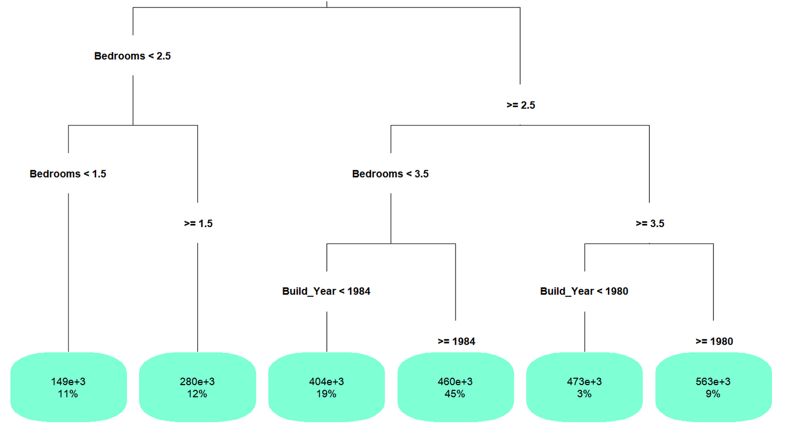
Surprisingly this decision tree was quite simple, even considering the small number of variables. Often, first iterations of decision trees can be highly complex and require ‘pruning’. The number of bathrooms and block size don’t feature in the tree so the ‘importance’ of these variables was reviewed.
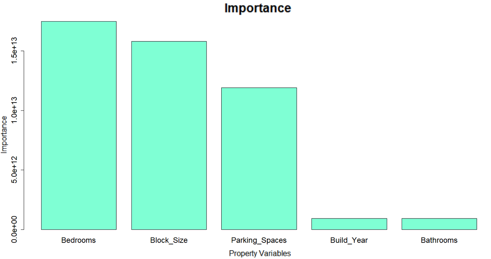 Variable importance for original binary decision tree.
As we can see, ‘Bedrooms’ was the most important variable followed closely by ‘Block Size’ and ‘Parking Spaces’ however the latter two variables did not appear in the tree. Earlier the default settings were used for the control parameters. These figures were adjusted to define the number of allowed layers in the decision tree as well as the minimum number of observations from the training set which need to fall into one of the final ‘leaves’ of the tree. All of the green boxes in the original decision tree represent leaves as there are no decisions made after these boxes. Each leaf represents a potential output from the model and if less than a defined number of observations from the training set arrive at this leaf, then the leaf is ‘pruned’ off the tree. This pruning reduces the likelihood of over-fitting as it keeps the model more simplistic and therefore general. It also reduces the complexity of the tree which allows it to run faster.
Once the control parameters were adjusted, a new tree was produced.
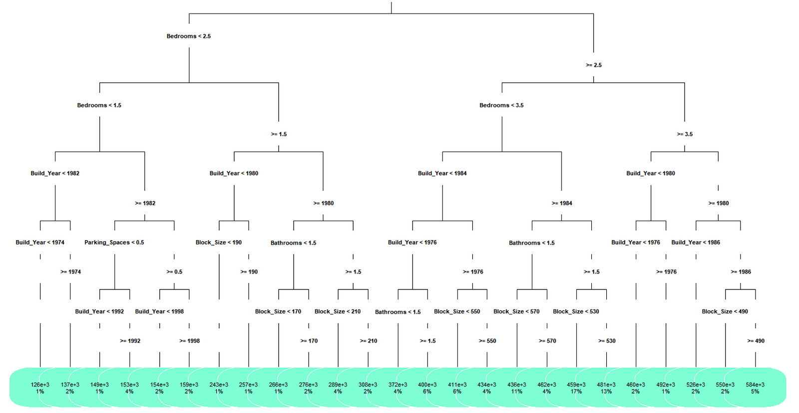 New decision tree with adjusted control parameters.
The new decision tree has become significantly more complex and now includes the ‘Block Size’ and ‘Bathroom’ variables. Root mean squared error (RMSE) is often used to determine the accuracy of machine learning algorithms. The second model was approximately 40% more accurate using this measure with the RMSE value for both the training and testing set being very similar suggesting the model isn’t over-fitting. Based on the accuracy improvement, the second tree would likely be a better alternative as it doesn’t appear to be unnecessarily complex and has provided a significant accuracy improvement.
The intent of this blog was to provide some clarification of how machine learning can be readily applied to solve real world problems. This simplistic Value prediction function was just one example where machine learning can be used to avoid building a potentially rigid and complex manual model and ultimately save time and effort. There are lots of great (and free!) resources online if this has whet your appetite to learn more!
Good luck!
Originally published at Towards Data Science


