Problem Solving as Data Scientist: a Case Study

There are two myths about how data scientists solve problems: one is that the problem naturally exists, hence the challenge for a data scientist is to use an algorithm and put it into production. Another myth considers data scientists always try leveraging the most advanced algorithms, the fancier model equals a better solution. While these are not fully groundless, they represent two common misunderstandings on how data scientists work: one emphasizes too much on the “execution” side, and the other overstate the “algorithm” part.

Obviously, these myths are not how we actually solve problems. From my perspective, problem-solving for a data scientist is:

more about “how to abstract the problem out of the business context”, not just “be handed with a specific task”
more about “solve the problem with an algorithm”, not just “use the best algorithm to solve a problem”
more about “iteratively deliver business value”, not just “implement the code and call it a day”.

With this said, I observe there are usually four stages involved in the problem-solving process, and I would like to share what are the four stages, and how it works in action with a case study, and then how can we get there with the right mindsets.

The story starts with, once upon a time …

My first job was in a company that operates an automotive pricing and information website and it went through the initial public offering (IPO) in May 2014. It was a great experience and I vividly remember everyone around was cheering on that day for the birth of a public company. As a public company, our revenue started to receive a lot of attention, especially with the first quarterly earnings report coming out in August. In early July, the director in the revenue department came to the Data Scientists’ seating area, and it did not look like he got good news to share.

“We are in trouble, a percentage of the sales revenue cannot be credited appropriately; we need your help.”

Here are some relevant contexts: the company’s revenue is generated based on the fact that it introduces more sales to car dealers. To get the deserved commission, we need to match the sale of a vehicle to the correct customer. If our data providers can tell us which customer bought which vehicle, then the matching is done and no extra effort is needed; however, the problem is that one data provider decided to not provide the 1-to-1 sale record: it has to be done in a batch (visualization on what is a “batch” shown as below), then it is much harder and uncertain to know which customer bought which car.

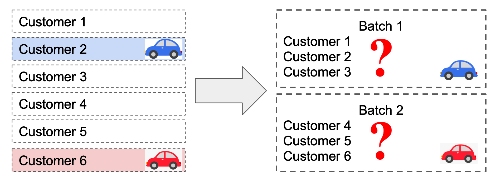
The revenue team was surprised by this change and after spending the past month trying to solve the problem, only 2% of sales from that data provider could be recovered manually. This would be bad news for the first earning call, so they came to seek help from Data Scientists. This is clearly an urgent problem that needs to be solved, so we jumped right on it.

Stage 1. understand the problem, and then redefine it using mathematical terms

This is the first stage of problem-solving in Data Science. Regarding “understand the problem” part, one needs to clearly identify the pain points so that once the pain point is resolved, the problem should be gone; regarding “redefine” the problem part, this is usually why a problem needs Data Scientist help.

For the specific one asked by our revenue team, the problem is: we cannot assign each sold vehicle to a customer, then we lose the revenue.

The pain point is: finding who purchased a vehicle in the given batch is manual and inaccurate, considering there are thousands of batches that need matching sales, it is very time-consuming and not sustainable.

The “redefined” problem in a mathematical term is: given a batch with customer C1, C2, .., Cn, along with the sold vehicle information, V1, V2, …, Vm, we need an automated solution to accurately identify the right matching pair (Ci, Vj) reflecting the actual purchasing event.

Stage 2. decompose the problem, identify a logical algorithm solution, and then build it out

With the redefined problem, we can see this is a “matching” exercise under constraint, with given customers and vehicles in a batch. So I decomposed the problem further into two steps:

Step 1. calculate the purchase likelihood for a customer given the vehicle P(C|V)
Step 2. based on the likelihood, attribute a car to the most likely customer in the batch

Now we can further identify the solution for each.

Step 1. probability calculation

For simplicity, let’s assume there are three customers (c1, c2, c3) in this batch, and one vehicle (v1) information is provided as a sale.

P(C=c1) represents the likelihood of c1 to buy any car. Assuming no prior knowledge about each customer, their likelihood of buying any car should be the same: P(C=c1) = P(C=c2) = P(C=c3), which equals a constant (e.g. 1/3 in this situation)
P(V=v1) is the likelihood for v1 to be sold, given it is shown in this batch, this should be 1 (100% likelihood to be sold)

Since there is only one customer making the purchase, this probability can be extended into:

P(V=v1) = P(C=c1, V=v1) + P(C=c2, V=v1) + P(C=c3, V=v1) = 1.0

For each of the item, given the following formula

P(C=c1, V=v1) = P(C=c1|V=v1) * P(V=v1) = P(V=v1|C=c1) * P(C=c1)

We can see P(C=c1|V=v1) is proportional to P(V=v1|C=c1). So now, we can get the formula for the probability calculation:

and the key is to get the probability for each P(V|C). Such a formula can be verbally explained as: the likelihood for a vehicle to be purchased by a specific customer is proportional to the likelihood for the customer to buy this specific vehicle.

The above formula may look too “mathematical”, so let me put it into an intuitive context: assuming three people were in a room, one is a musician, one is an athlete, and one is a data scientist. You were told there is a violin in this room belong to one of them. Now guess, whom do you think is the owner of the violin? This is pretty straightforward, right? given the likelihood of musician to own a violin is high, and the likelihood of athlete and data scientists to own a violin is lower, it is much more likely for the violin to belong to the musician. The “mathematical” thinking process is illustrated below.

Now, let’s put the probabilities into a business context. As an online automotive pricing platform, each customer needs to generate at least one vehicle quote, hence, we assume the customer can be reasonably represented as the vehicles he/she quoted. Then such P(V|C) probability can be learned from existing data the company already accumulated in the history, including who generated a vehicle quote at when, and what vehicle they eventually bought. I would not further elaborate on the details, but the key point is that we can learn P(V|C), and then calculate the needed probability P(C|V) in each batch.

Step 2. vehicle attribution

Once we get the expected probability for each vehicle to be sold to customers, the second step is the attribution process. Assuming there is only one sold vehicle in the batch, such process is trivial; however, if there are multiple sold vehicles in the batch, either following approaches would work:

(direct attribution) use only the calculated probability P(C|V), always attribute vehicle to customers with the highest likelihood. Under this approach, it is possible to attribute two vehicles to the same customer.
(round-robin way) assume each customer buys at most one vehicle: once one vehicle is attributed to a customer, both are removed before the next round vehicle attribution.

Now we have designed a two-stepped algorithm to solve the key challenge, and it’s time to test the performance! Given there are historic quotes and sales data, it is straightforward to simulate the process of “creating random batches”, “attaching sales to the batch”, and try to “recover sales from the given batch information”. Such simulation provides a way to evaluate the model’s performance and we estimated more than 50% of sales can be recovered with high precision (>95%). We deployed the model for the real dataset, and the results matched our expectations well.

The revenue team was very happy with the above solution: comparing to the ~2% recovery rate, 50% is more than 25 X! From a business impact perspective, this revenue directly added to the bottom line for our first quarterly earnings report, and the contributed value from the Data Science team is significant.

Stage 3. Think deeper, and seek opportunities to make further improvement

We run the above solution for an extra month and see the performance is pretty consistent, and now it is time to think about what’s next? We recovered 50% of sales, but how about the rest 50%? Is it possible to further improve the algorithm to get there?

Usually, we, as data scientists, have a tendency to focus too much on the algorithm details; in this case, there were some discussions around how to better model the P(V|C): should we use a deep learning model to make this probability much better, etc. However, per my understanding, these pure algorithmic improvements usually result in just incremental performance, and it’s less likely we close the rest 50% gap.

Then I started a deeper conversation with the revenue team and trying to figure out what was missing in our understanding about the problem, turns out we can control how the customers are grouped into a batch! Although there are some restrictions (e.g. customers have to generate quotes from the same dealership), this gives us the freedom to further optimize, and I see this is the direction to close the gap of the rest 50% sales.

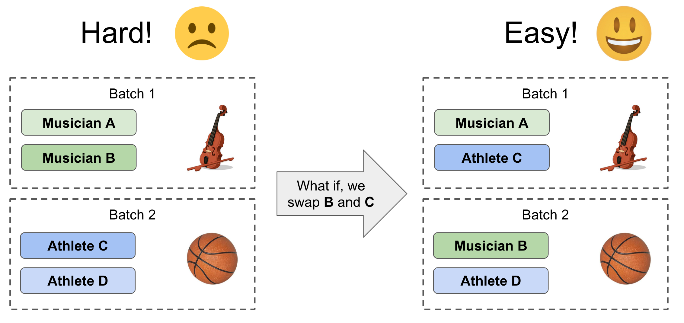
Why am I confident in this direction? Think about this situation: if you have 4 people to be batched, and each batch has 2 people. The best batching strategy is to put the most different people in the same batch so that once an item is returned, the attribution will be more accurate. The following visualization shows the concept. On the left side, if you put two musicians in the same batch, two athletes in the same batch, it’s very hard to know who owns the violin or basketball. While on the right side, if you have each batch with one musician and one athlete, it is much easier to tell Musician A owns the violin, and Athlete D owns the basketball, with high confidence.

To materialize the above concept, there are two steps required:

(similarity definition) how to define customer to customer similarity? and then a batch’s entropy as the objective function to optimize for?
(batch optimization) based on the above similarities, how to design an optimization strategy to achieve optimal batches?

Step 1. similarity definition

In the first stage solution, we already find a way to calculate P(V|C), here, I would make a direct generalization: the similarity between two customers is proportional to the average likelihood for both customers to purchase each other’s quoted vehicles. If each customer quoted only one vehicle (c1 quoted v1, and c2 quoted v2), then a simplified version looks as follows:

Similarity(C1, C2) = 0.5 * (P(V=v1|C=c2) + P(V=v2|C=c1))

Once we have the pairwise similarity between two customers, we can define the entropy for a batch as the sum of mutual pairwise similarities between customers in the batch. Now, we have an objective function to optimize for: we want batches with maximum entropy

Step 2. batch optimization

After reading some similar studies, I decided to use the 2-opt algorithm, which is a simple local search algorithm for solving the traveling salesman problem.

The basic concept of 2-opt algorithm is as follows: in every step, two edges are randomly picked and attempt to “swap”, if the objective function is better after the swap is done, then the swap will be executed; or else, re-pick two edges. The algorithm continues until the objective function is converged or the maximum iteration number is met. The following figure illustrates when two edges (red) are picked and swapped into new edges (blue), achieving a shorter distance.

To apply the 2-opt algorithm in my case, I made analogies to the traveling salesman problem (TSP):

In TSP, two edges are randomly selected; in my cases, two batches are randomly selected, and then each batch randomly pick one customer inside to exchange
In TSP, the total distance is used as the objective function, the shorter the better; in my case, the entropy of all batches is the objective function, the higher the better.

Great, we have all the elements to optimize the batches! After implementing the algorithm, we further backtest over the existing data and found that: more than 85% of sales could be recovered. In the following month, when we apply this over the real dataset, the recovery rate is found at a similar level. This approach works, as expected!

Stage 4. Engineering the solution to make it extendable and maintainable

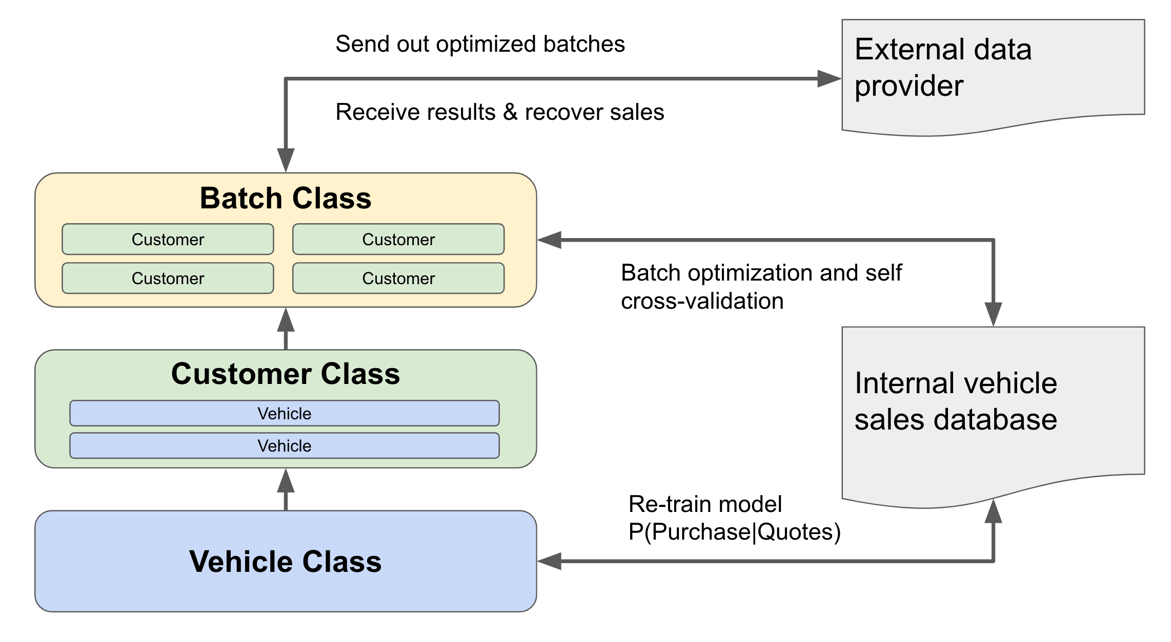
What I described above is mainly the algorithm design part; and in parallel, there is the Engineering development part, and it is not easy to simply write the code and expect it to be extendable and maintainable.

During the project evolution, we gradually noticed there is a pattern of dependencies across the modules needed. The vehicle is represented by many features, and the customer is represented by a set of vehicles, and the batch is represented by a set of customers. With this high-level representation, we can build the dependency lineage as Vehicle -> Customer -> Batch.

Meanwhile, as a data product, we need to make sure the system can evolve to update the needed parameters and always evaluate the performance along the way. Hence the architecture was designed in the following way

The general problem-solving flow with the right mindset

The data science area is quite broad and designing algorithmic data products is only part of many potential projects. Other commonly-seen data science projects are experimentation design, causal inference, deep-dive analysis to drive strategic changes, etc. Although they may not strictly follow or even need all the stages I listed above, the four-stage flow still help to lay out a way to think about problem-solving in general:

Stage 1 (problem identification) is to help you focus on the key question and not loose track while diving deep into data
Stage 2 (first logical solution) is to get you a quick win and keep the momentum to build trust with business partners
Stage 3 (iterative improvement) is to help you move the solution further ahead and be the owner of the area
Stage 4 (operational excellence) is to help you remove tech debt, to set you free from mundane maintenance works going forward

The four-stage flow is not necessarily a strict rule one should follow, but it is more like a natural outcome if a data scientist has the right mindsets while facing any incoming challenge. In my opinion, these mindsets are:

Business-driven, not algorithm-driven. Look at the big picture and see how data science fits in the business, understand why data science is needed and how it delivers value. Don’t be too attached to any specific algorithm: “if all you have is a hammer, everything looks like a nail”.
Owning the problem, not just taking orders. Being the owner of a problem means one will be proactive in thinking about how to solve it now, solve it better, and solve it with less effort. One would not stop at a sub-optimal solution and consider it done.
Open-minded, and always be learning. As an interdisciplinary field, data science overlaps with statistics, computer science, operational research, psychology, economics, marketing, sales, and more! It’s almost impossible to know all the areas ahead of time, so be open-minded and keep learning along the way. There could always be a better solution than the one you already knew.

Hope you may find the above sharing helpful: happy problem solving, the data science way.