How to not be fooled by the tricks data plays on you.
Dataset shift is a challenging situation where the joint distribution of inputs and outputs differs between the training and test stages. — Dataset Shift, The MIT Press.
Dataset shifting is one of those topics which is simple, perhaps so simple that it is considered trivially obvious. In my own data science classes the idea was discussed briefly, however, I think a deeper discussion of the causes and manifestations of dataset shift are of benefit to the data science community.
The key theme of this article can be summarized in a single sentence:
Dataset shift is when the training and test distributions are different.


Whilst you may scoff at the triviality of such a statement, this is possibly the most common problem I see when viewing solutions to Kaggle challenges. In some ways, a deep understanding of dataset shifting is key to winning Kaggle competitions.
Dataset shift is not a standard term and is sometimes referred to as concept shift or concept drift, changes of classification, changing environments, contrast mining in classification learning, fracture points and fractures between data.
Dataset shifting occurs predominantly within the machine learning paradigm of supervised and the hybrid paradigm of semi-supervised learning.
The problem of dataset shift can stem from the way input features are utilized, the way training and test sets are selected, data sparsity, shifts in the data distribution due to non-stationary environments, and also from changes in the activation patterns within layers of deep neural networks.
Why is dataset shift important?
It is application-dependent and thus relies largely on the skill of the data scientist to examine and resolve. For example, how does one determine when the dataset has shifted sufficiently to pose a problem to our algorithms? If only certain features begin to diverge, how do we determine the trade-off between the loss of accuracy by removing features and the loss of accuracy by a misrepresented data distribution?
In this article, I will discuss the different types of dataset shift, problems that can arise from their presence, and current best practices that one can use to avoid them. This article contains no code examples and is purely conceptual. Classification examples will be used for ease of demonstration.
There are multiple manifestations of dataset shift that we will examine:
- Covariate shift
- Prior probability shift
- Concept shift
- Internal covariate shift (an important subtype of covariate shift)
This is a huge and important topic in machine learning so do not expect a comprehensive overview of this area. If the reader is interested in this subject then are a plethora of research articles on the topic — the vast majority of which focus on covariate shift.
Covariate shift
Of all the manifestations of dataset shift, the simplest to understand is covariate shift.
Covariate shift is the change in the distribution of the covariates specifically, that is, the independent variables. This is normally due to changes in state of latent variables, which could be temporal (even changes to the stationarity of a temporal process), or spatial, or less obvious. — Quora
Covariate shift is the scholarly term for when the distribution of the data (i.e. our input features) changes.

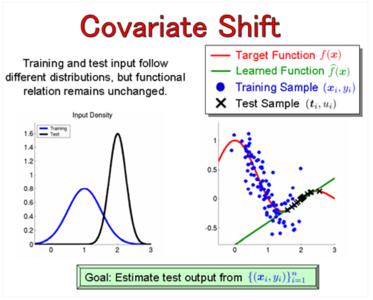
Here are some examples where covariate shift is likely to cause problems:
- Face recognition algorithms that are trained predominantly on younger faces, yet the dataset has a much larger proportion of older faces in it.
- Predicting life expectancy but having very few samples in the training set of individuals that smoke, and many more samples of this in the training set.
- Classifying images as either cats or dogs and omitting certain species from the training set that are seen in the test set.
In this case, there is no change in the underlying relationship between the input and output (the regression line is still the same), yet part of that relationship is data-sparse, omitted, or misrepresented such that the test set and training set do not reflect the same distribution.
Covariance shift can cause a lot of problems when performing cross-validation. Cross-validation is almost unbiased without covariate shift but it is heavily biased under covariate shift!
Prior Probability Shift
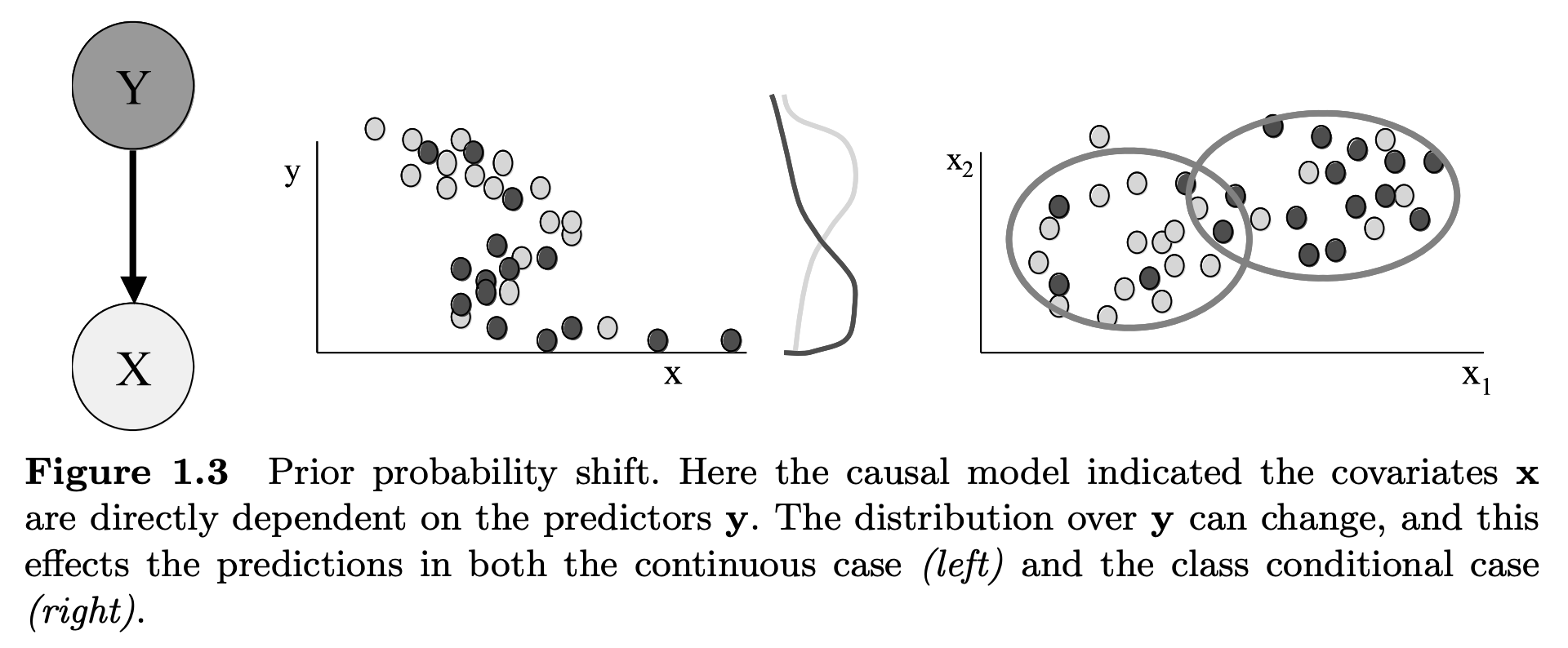
Whilst covariate shift focuses on changes in the feature (x) distribution, prior probability shift focuses on changes in the distribution of the class variable y.


This type of shifting may seem slightly more confusing but is it essentially the reverse of covariate shift. An intuitive way to think about it might be to consider an unbalanced dataset.
If the training set has equal prior probabilities on the number of spam emails that you receive (i.e. the probability of an email being spam is 0.5), then we would expect 50% of the training set to contain spam emails and 50% to contain non-spam.
If, in reality, only 90% of our emails are spam (perhaps not unlikely), then our prior probability of the class variables has changed. This idea has relations to data sparsity and biased feature selection that are factors in causing covariance shift, but instead of influencing our input distribution, they instead influence our output distribution.
This problem only occurs in Y → X problems and is commonly associated with naive Bayes (hence the spam example, since naive Bayes is commonly used to filter spam emails).
The below figure on prior probability shift is taken from the Dataset Shift in Machine Learning book and illustrates this case nicely.
Concept Drift
Concept drift is different from covariate and prior probability shift in that it is not related to the data distribution or the class distribution but instead is related to the relationship between the two variables.
An intuitive way to think about this idea is by looking at time series analysis.
In time series analysis, it is common to examine whether the time series is stationary before performing any analysis, as stationary time series are much easier to analyze than non-stationary time series.
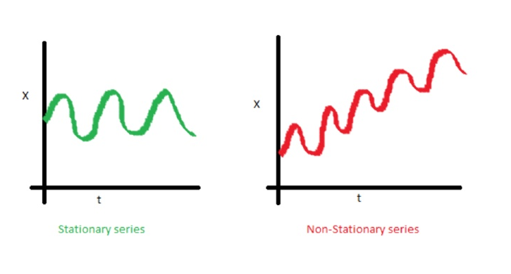
Why is this the case?
This is easier because the relationship between the input and output is not consistently changing! There are ways of detrending a time series to make it stationary, but this does not always work (such as in the case of stock indices that generally contain little autocorrelation or secular variation).

To give a more concrete example, let’s say we examined the profits of companies before the 2008 financial crisis and made an algorithm to predict the profit based on factors such as the industry, number of employees, information about products, and so on. If our algorithm is trained on data from 2000–2007, but are not using it to predict the same information after the financial crisis, it is likely to perform poorly.
So what changed? Clearly, the overall relationship between the inputs and outputs changed due to the new socio-economic environment, and, if these are not reflected in our variables (such as having a dummy variable for the date that the financial crisis occurred and training data before and after this date) then our model is going to suffer the consequences of concept shift.
In our specific case, we would expect to see profits change markedly in the years after the financial crisis (this is an example of an interrupted time series).
Internal Covariate Shift
One reason this topic has gained interest recently is due to the suspected influence of covariance shift in the hidden layers of deep neural networks (hence the word ‘internal’).
Researchers found that due to the variation in the distribution of activations from the output of a given hidden layer, which are used as the input to a subsequent layer, the network layers can suffer from covariate shift which can impede the training of deep neural networks.
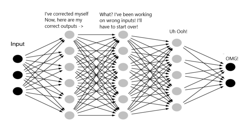
The situation without batch normalization, network activations are exposed to varying data input distributions that propagate through the network and distort the learned distributions.
This idea is the stimulus of batch normalization, proposed by Christian Szegedy and Sergey Ioffe in their 2015 paper “Batch Normalization: Accelerating Deep Network Training by Reducing Internal Covariate Shift”.
The authors propose that internal covariate shift in the hidden layers slows down training and requires lower learning rates and careful parameter initialization. They resolve this by normalizing the inputs to hidden layers by adding a batch normalization layer.
This batch norm layer takes the mean and standard deviation of a batch of samples and uses them to standardize the input. This also adds some noise to the inputs (because of the noise inherent in the mean and standard deviation between different batches) which helps to regularize the network.

How batch normalization fits within the network architecture of deep neural networks.
This problem acts to translate the varying distribution to more stable internal data distributions (less drift/oscillations) that helps to stabilize learning.
Varying data distributions across batches are normalized via a batch normalization layer in order to stabilize the data distribution used as input to subsequent layers in a deep neural network.
Batch normalization is now well adopted in the deep learning community, although a recent paper alluded that the improved results obtained from this technique may not be purely due to the suppression of internal covariate shift, and may instead be a result of smoothing the loss landscape of the network.
For those unfamiliar with batch normalization, its purpose, and its implementation, I recommend looking at the relevant Youtube videos of Andrew Ng, one of which is linked below.
Major Causes of Dataset Shift
The two most common causes of dataset shift are (1) sample selection bias and (2) non-stationary environments.
It is important to note that these are not types of dataset shift, and do not always result in dataset shift. They are merely potential reasons that dataset shift can occur in our data.
Sample selection bias: the discrepancy in distribution is due to training data having been obtained through a biased method, and thus do not represent reliably the operating environment where the classifier is to be deployed (which, in machine learning terms, would constitute the test set).
Non -stationary environments: when the training environment is different from the test one, whether it is due to a temporal or a spatial change.
Sample Selection Bias
Sample selection bias is not a flaw with any algorithm or handling of the data. It is purely a systematic flaw in the process of data collection or labeling which causes nonuniform selection of training examples from a population, which causes biases to form during training.
Sample selection bias is a form of covariance shift since we are influencing our data distribution.
This can be thought of as a misrepresentation of the operating environment such that our model optimizes its training environment to a factitious or cherry-picked operating environment.

Dataset shift resulting from sample selection bias is especially relevant when dealing with imbalanced classification, because, in highly imbalanced domains, the minority class is particularly sensitive to singular classification errors, due to the typically low number of samples it presents.
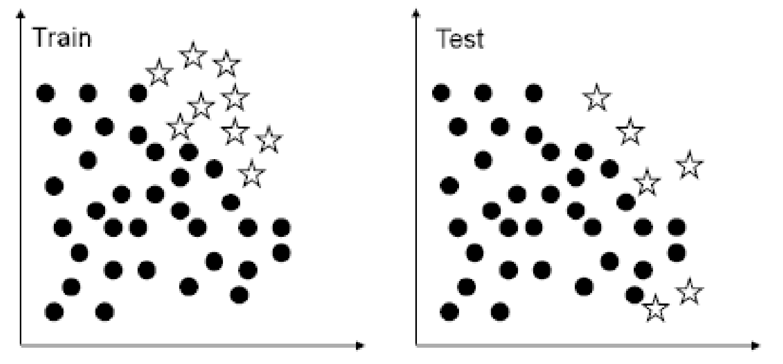
Example of the impact of dataset shift in imbalanced domains.
In the most extreme cases, a single misclassified example of the minority class can create a significant drop in performance.
Non -stationary environments
In real-world applications it world applications, it is often the case that the data is not (time- or space-) stationary.
One of the most relevant non-stationary scenarios involves adversarial classification problems, such as spam filtering and network intrusion detection.
This type of problem is receiving an increasing increasing amount of attention in the machine learning field and usually copes with non-stationary environments due to the existence of an adversary that tries to work around the existing classifier’s learned concepts. In terms of the machine learning task, this adversary warps the test set so that it becomes different from the training set, thus introducing any possible kind of dataset shift.
Identifying Dataset Shift
There are several methods that can be used to determine whether shifting is present in a dataset and its severity.

Tree diagram showing the methods of identifying dataset shift.
Unsupervised methods are perhaps the most useful ways of identifying dataset shift, as they do not require post-hoc analysis to be done, the latency of which cannot be afforded in some production systems. Supervised methods exist which essentially look at growing errors as the model runs and the performance on an external holdout (validation set).
Statistical Distance The statistical distance method is useful for detecting if your model predictions change over time. This is done by creating and using histograms. By making histograms, you are not only able to detect whether your model predictions change over time, but also check if your most important features change over time. Simply put, you form histograms of your training data, keep track of them over time, and compare them to see any changes. This method is used commonly by financial institutions on credit-scoring models.
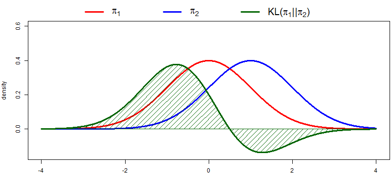
Two distributions are their KL-divergence (effectively the ‘distance’ between the two distributions). If the two distributions overlap, they are effectively the same distribution and the KL-divergence is zero.
There are several metrics which can be used to monitor the change in model predictions over time. These include the Population Stability Index (PSI), Kolmogorov-Smirnov statistic, Kullback-Lebler divergence (or other f-divergences), and histogram intersection.
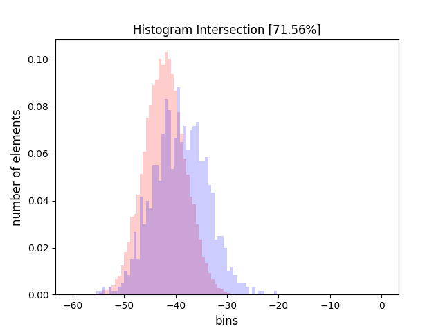
Data plotted along one feature axis for a training and test set. There is ~72% intersection of the distributions which indicates a reasonable level of covariate shift between the distributions.
The major disadvantage of this method is that is not great for high-dimensional or sparse features. However, it can be very useful and in my opinion should be the first thing to try when dealing with this issue.
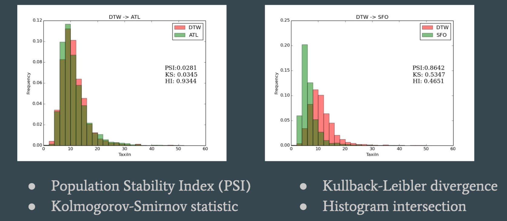
A comparison between KL-divergence, KS statistic, PSI, and histogram intersection for two examples. The left example shows little to no covariate shift, whilst the right example shows a substantial covariate shift. Notice how it affects the expected values of the statistical distances.
2) Novelty Detection A method that is more amenable to fairly complex domains such as computer vision, is novelty detection. The idea is to create a model for modeling source distribution. Given a new data point, you try to test what is the likelihood that this data point is drawn from the source distribution. For this method, you can use various techniques such as a one-class support vector machine, available in most common libraries.
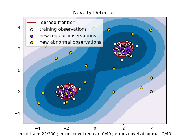
If you are in a regime of homogenous but very complex interactions (e.g. visual, audio, or remote sensing), then this is a method you should look into, because in that case, the statistical distance (histogram method) won’t be as effective a method.
The major disadvantage of this method is that it cannot tell you explicitly what has changed, only that there has been a change.
3) Discriminative Distance The discriminative distance method is less common, nonetheless, it can be effective. The intuition is that you want to train a classifier to detect whether or not an example is from the source or target domain. You can use the training error as proxy of the distance between those two distributions. The higher the error, the closer they are (i.e. the classifier cannot discriminate between the source and target domain).
Discriminative distance is widely applicable and high dimensional. Though it takes time and can be very complicated, this method is a useful technique if you are doing domain adaptation (and for some deep learning methods, this may be the only feasible technique that exists).
This method is good for high-dimensional and sparse data, and is widely applicable. However, it can only be done offline and is more complicated to implement than the previous methods.
Handling Dataset Shift
How do you correct dataset shift? If possible, you should always retrain. Of course, in some situations, it may not be possible, for example, if there are latency problems with retraining. In such cases, there are several techniques for correcting dataset shift.
1) Feature Removal
By utilizing the statistical distance methods discussed above which are used to identify covariate shift, we can use these as measures of the extent of the shifting. We can set a boundary on what is deemed an acceptable level of shift, and analyzing individual features or through an ablation study, we can determine which features are most responsible for the shifting and remove these from the dataset.
As you may expect, there is a trade-off between removing features that contribute to the covariate shift and having additional features and tolerating some covariate shift. This trade-off is something that the data scientist would need to assess on a case-by-case basis.
A feature that differs a lot during training and test, but does not give you a lot of predictive power, should always be dropped.
As an example, PSI is used in risk management and an arbitrary value of 0.25 is used as the limit, above which this is deemed as a major shift.
2) Importance Reweighting The main idea with importance reweighting is that you want to upweight training instances that are very similar to your test instances. Essentially, you try to change your training data set such that it looks like it was drawn from the test data set. The only thing required for this method is unlabeled examples for the test domain. This may result in data leakage from the test set.

On the left, we have our typical training set and in the center our test set. We estimate the data probability of the training and test sets and use this to rescale our training set to produce the training set on the right (notice the size of the points has got larger, this represents the ‘weight’ of the training example).
To make it clear how this works, we basically reweight each of the training examples by the relative probability of the training and test set. We can do this by density estimation, through kernel methods such as kernel mean matching, or through discriminative reweighting.
3) Adversarial Search
The adversarial search method uses an adversarial model where the learning algorithm attempts to construct a predictor that is robust to the deletion of features at test time.
The problem is formulated as finding the optimal minimax strategy with respect to an adversary which deletes features and shows that the optimal strategy may be found by either solving a quadratic program or using efficient bundle methods for optimization.
Covariate shift has been extensively studied in the literature, and a number of proposals to work under it have been published. Some of the most important ones include:
- Weighting the log-likelihood function (Shimodaira, 2000)
- Importance weighted cross-validation (Sugiyama et al, 2007 JMLR)
- Integrated optimization problem. Discriminative learning. (Bickel et al, 2009 JMRL)
- Kernel mean matching (Gretton et al., 2009)
- Adversarial search (Globerson et al, 2009)
- Frank-Wolfe algorithm (Wen et al., 2015)
Final Comments
Dataset shift is a topic that is, in my estimation, extremely important and yet undervalued by people in the field of data science and machine learning.
Given the impact it can have on the performance of our algorithms, I suggest spending some time working out how to handle data properly in order to give you more confidence in your models, and, hopefully, superior performance.
References
[1] http://iwann.ugr.es/2011/pdf/InvitedTalk-FHerrera-IWANN11.pdf
[2] J.G. Moreno-Torres, T. Raeder, R. Alaiz-Rodríguez, N.V. Chawla, F. Herrera. A Unifiying view of Data Shift in Classification. Pattern Recognition, 2011, In press.
[3] J. Quiñonero Candela, M. Sugiyama, A. Schwaighofer, and N. D. Lawrence. Dataset Shift in Machine Learning Shift in Machine Learning. The MIT Press 2009 The MIT Press, 2009.
[4] Raeder, Hoens & Chawla. Consequences of Variability in Classifier of Variability in Classifier Performance Estimates., ICDM ’10 Proceedings of the 2010 IEEE International Conference on Data Mining.
[5] Moreno-Torres, J. G., & Herrera, F. (2010). A preliminary study on overlapping and data fracture in imbalanced domains by means of genetic programming-based feature extraction. In Proceedings of the 10th International Conference on Intelligent Systems Design and Applications (ISDA 2010) (pp. 501–506).
[6] https://www.ncbi.nlm.nih.gov/pmc/articles/PMC5070592/pdf/f1000research-5-10228.pdf

