Tutorial (including R code) for using Generalized Estimating Equations and Multilevel Models.
While regression models are easy to run given their short, simple syntax, this accessibility also makes it easy to use regression inappropriately. These models have several key assumptions that need to be met in order for their output to be valid, but your code will typically run whether or not these assumptions have been met.
For linear regression (used with a continuous outcome), these assumptions are as follows:
- Independence: All observations are independent of each other, residuals are uncorrelated
- Linearity: The relationship between X and Y is linear
- Homoscedasticity: Constant variance of residuals at different values of X
- Normality: Data should be normally distributed around the regression line
For logistic regression (used with a binary or ordinal categorical outcome), these assumptions are as follows:
- Independence: All observations are independent of each other, residuals are uncorrelated
- Linearity in the logit: The relationship between X and the logit of Y is linear
- Model is correctly specified, including lack of multicollinearity
In both kinds of simple regression models, independent observations are absolutely necessary to fit a valid model. If your data points are correlated, this assumption of independence is violated. Fortunately, there are still ways to produce a valid regression model with correlated data.
Correlated Data
Correlation in data occurs primarily through multiple measurements (e.g. two measurements are taken on each participant 1 week apart, and data points within individuals are not independent) or if there is clustering in the data (e.g. a survey is conducted among students attending different schools, and data points from students within a given school are not independent).
The result is that that the outcome has been measured on the level of an individual observation, but that there is a second level of either an individual (in the case of multiple time points) or clusters on which individual data points can be correlated. Ignoring this correlation means that standard error cannot be accurately computed, and in most cases will be artificially low.
The best way to know if your data is correlated is simply through familiarity with your data and the collection process that produced it. If you know that you have repeated measures from the same individuals or have data on participants who can be grouped into families or schools, you can assume that your data points are probably not independent. You can also investigate your data for possible correlation by calculating the ICC (intraclass correlation coefficient) to determine how correlated data points are within possible groups, or by looking for correlation in your residuals.
Regression Modeling with Correlated Data
As previously mentioned, simple regression will produce inaccurate standard errors with correlated data and therefore should not be used.
Instead, you want to use models that can account for the correlation that is present in your data. If the correlation is due to some grouping variable (e.g. school) or repeated measures over time, then you can choose between Generalized Estimating Equations or Multilevel Models. These modeling techniques can handle either binary or continuous outcome variables, so can be used to replace either logistic or linear regression when the data are correlated.
Generalized Estimating Equations
Generalized estimating equations (GEE) will give you beta estimates that are the same or similar to those produced by simple regression, but with appropriate standard errors. Generalized estimating equations are particularly useful when you have repeated measures for the same individuals or units. This modeling technique tends to work well when you have many small clusters, which is often the result of having a few measurements on a large number of participants. GEE also allows the user to specify one of numerous correlation structures, which can be a useful feature depending on your data.
Multilevel Modeling
Multilevel modeling (MLM) also provides appropriate standard errors when data points are not independent. It is typically the best modeling approach when the user is interested in relationships both within and between clustered groups, and is not simply looking to account for the effect of correlation in standard error estimates. MLM has the additional advantage of being able to handle more than two levels in the response variable. The primary drawback of MLM models is that they require larger sample sizes within each cluster, so may not work well when clusters are small.
Both GEE and MLM are fairly easy to use in R. Below, I will walk through examples with the two most common kinds of correlated data: data with repeated measures from individuals and data collected from individuals with an important grouping variable (in this case, country). I will fit simple regression, GEE, and MLM models with each dataset, and will discuss which modeling technique is best for these different data types.
Example 1: Data from the Fragile Families & Child Wellbeing Study
The data that I will be working with first comes from Years 9 and 15 of the Princeton University Fragile Families & Child Wellbeing Study, which follows the families of selected children born between 1998 and 2000 in major US cities. Data are publicly available, and can be accessed by submitting a brief request on the Fragile Families Data and Documentation page. Since this study follows up with the same families year after year, data points from the same family units at different time points are not independent.
This dataset contains dozens of variables representing the health of wellbeing of participating children and their parents. Being in psychiatric epidemiology, I am primarily interested in examining the children’s mental-wellbeing. Participating children are asked if they frequently feel sad, and I will be using answers to this “often feeling sad” question as my outcome. Since substance use is tied to poorer mental wellbeing among adolescents, I will be using variables representing alcohol and tobacco use as predictors*.
*Note: Models created in this article are for demonstration purposes only and should not be considered to be meaningful. I have not considered confounding, mediation, other model assumptions, or other possible data issues in the construction of these models.
First, let’s load the packages that we’ll be using. I’ve loaded “tidyverse” to clean our data, “haven” because the data we’ll be reading in comes in SAS format, “geepack” to run our GEE model, and “lme4” to run our multilevel model:
library(tidyverse)
library(haven)
library(geepack)
library(lme4)
Now let’s do some data cleaning to get these data ready for modeling!
Data from Years 9 and 15 are housed in separate SAS files (identifiable by the .sas7bdat extension), so we have one code chunk to read in and clean each file. This cleaning has to be done separately because variable names and coding differ slightly between study years (see the Data and Documentation page for codebooks).
There are hundreds of variables included in the datasets, so we first select those that will be used in our model and assign meaningful variable names that are consistent across data frames. Next, we filter the data to only include individuals with complete data for our variables of interest (the code below excludes individuals with missing data for these variables as well as those who refused to answer).
We then recode our variables in the standard 1 = “yes”, 0 = “no” format. For the “feel_sad” variable, this also means dichotomizing a variable with 4 levels which represent varying degrees of sadness. We end up with a binary variable where 1 = “sad” and 0 = “not sad.” Some regression techniques can handle multiple levels in your response variable (MLM included), but I have binarized it here for simplicity. Finally, we create a “time_order” variable indicating if the observation comes from the first or second round of the study.
year_9 = read_sas("./data/FF_wave5_2020v2_SAS.sas7bdat") %>%
  select(idnum, k5g2g, k5f1l, k5f1j) %>%
  rename("feel_sad" = "k5g2g",
         "tobacco" = "k5f1l",
         "alcohol" = "k5f1j") %>%
  filter(
    tobacco == 1 | tobacco == 2,
    alcohol == 1 | alcohol == 2,
    feel_sad == 0 | feel_sad == 1 | feel_sad == 2 | feel_sad == 3
  ) %>%
  mutate(
    tobacco = ifelse(tobacco == 1, 1, 0),
    alcohol = ifelse(alcohol == 1, 1, 0),
    feel_sad = ifelse(feel_sad == 0, 0, 1),
    time_order = 1
  )year_15 = read_sas("./data/FF_wave6_2020v2_SAS.sas7bdat") %>%
  select(idnum, k6d2n, k6d40, k6d48) %>%
  rename("feel_sad" = "k6d2n",
         "tobacco" = "k6d40",
         "alcohol" = "k6d48") %>%
  filter(
    tobacco == 1 | tobacco == 2,
    alcohol == 1 | alcohol == 2,
    feel_sad == 1 | feel_sad == 2 | feel_sad == 3 | feel_sad == 4
  ) %>%
  mutate(
    tobacco = ifelse(tobacco == 1, 1, 0),
    alcohol = ifelse(alcohol == 1, 1, 0),
    feel_sad = ifelse(feel_sad == 4, 0, 1),
    time_order = 2
  )
We then combine data from Years 9 and 15 by stacking our two cleaned data frames using rbind(). The rbind() function works well here because both data frames now share all variable names. We next transform the “idnum” variable (which identifies unique family units) into a numeric variable so that it can be properly used to sort the data in the final code chunk. This step is necessary because the geeglm() function that we will be using to run the GEE model assumes that the data frame is sorted first by a unique identifier (in this case, “idnum”), and next by the order of observations (indicated here by the new “time_order” variable).
fragile_families = rbind(year_9, year_15) %>%
  mutate(
    idnum = as.numeric(idnum)
  )fragile_families =
  fragile_families[
  with(fragile_families, order(idnum)),
]
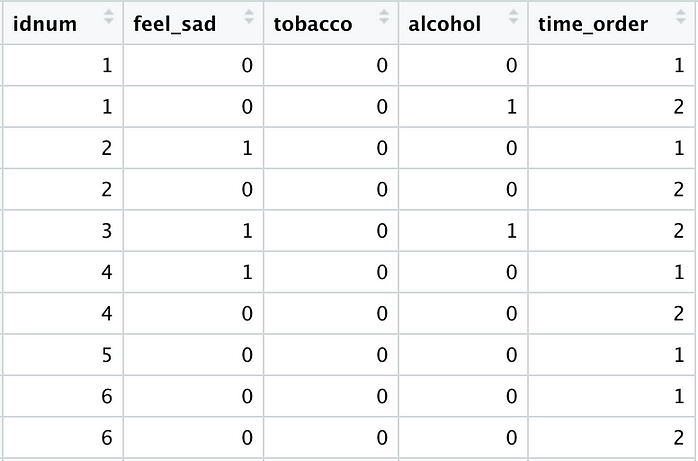
The above code produces the following cleaned data frame, which is now ready to be used for regression modeling:
Let’s fit our models:
- Simple Logistic Regression
First, we use the glm() function to fit a simple logistic regression model using the “fragile_families” data. Since we have a binary outcome variable, “family = binomial” is used to specify that logistic regression should be used. We also use tidy() from the “broom” package to clean up the model output. We are creating this model for comparison purposes only — as indicated before, the independence assumption has been violated and the standard errors associated with this model will not be valid!
glm(formula = feel_sad ~ tobacco + alcohol,
    family = binomial, data = fragile_families) %>%
  broom::tidy()
The above code produces the following output, which the subsequent modeling approaches will be compared to. Tobacco and alcohol use both appear to be significant predictors of sadness in participating children.

2. Generalized Estimating Equations
The syntax used to specify a GEE model using the geeglm() function from the “geepack” package is fairly similar to that used with the standard glm() function. The “formula”, “family”, and “data” are arguments are exactly the same for both functions. What’s new are the “id,” “waves,” and “corstr” arguments (see package documentation for all available arguments). The unique identifier that links observations from the same subject is specified in the “id” argument. In this case the ID is “idnum,” the unique identifier assigned to each family participating in the study. The “time_order” variable created during data cleaning comes into play in the “waves” argument, where it indicates the order in which observations were made. Finally, “corstr” can be used to specify the within-subject correlation structure. “Independence” is actually the default input for this argument, and it makes sense in this context because it is useful when clusters are small. However, “exchangeable” can be specified when all observations within a subject can be considered to be equally correlated, and “ar1” is best when the internal correlations change over time. Information on choosing the right correlation structure can be found here and here.
geeglm(formula = feel_sad ~ tobacco + alcohol,
       family = binomial, id = idnum, data = fragile_families,
       waves = time_order, corstr = "independence") %>%
  broom::tidy()
Our GEE model gives us the following output:

As you can see, our beta estimates are exactly the same as those produced using glm(), but standard error differs slightly now that the correlations in the data have been accounted for. While tobacco and alcohol are still significant predictors of sadness, the p-values are somewhat different**. If these p-values were closer to 0.05, having accurate standard error measurements could easily push a p-value over or under the level of significance.
**Note: The test statistics for GEE and logistic regression look drastically different, but this is only because the test statistic provided in the logistic regression output is a Z-statistic and the test statistic provided in the GEE output is a Wald statistic. The Z-statistic is calculated by dividing the estimate by the standard error, while the Wald statistic is calculated by squaring the result of dividing the estimate by the standard error. The two values are therefore mathematically related, and by taking the square root of the values in the GEE “statistic” column you will see a much more moderate change from the initial Z-statistics.
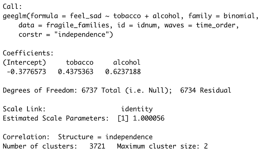
With the geeglm() function, it is also important to verify that your clusters have been properly recognized. You can do this by running the above code without the broom::tidy() step, so:
geeglm(formula = feel_sad ~ tobacco + alcohol,
       family = binomial, id = idnum, data = fragile_families,
       waves = time_order, corstr = "independence")
This code produces the output shown below. You want to look to the last line of the output, where “Number of clusters” and “Maximum cluster size” are described. We had 2 observations for several thousand individuals, so these values make sense in the context of our data and indicate that clusters were registered correctly by the function. If, however, the number of clusters is equal to the number of rows in your dataset, something is not working properly (most likely the sorting of your data is off).
3. Multilevel Modeling
Next, let’s fit a multilevel model using glmer() from the lme4 package. Again, the required code is almost identical to that used for logistic regression. The only required change is specifying random slopes and intercepts in the formula argument. This is done with the “(1 | idnum)” bit of code, which follows the following structure: (random slopes | random intercepts). The grouping variable, in this case “idnum,” is specified to the right of the | as “random intercepts,” and the “1” indicates that we don’t want the predictors’ effects to vary across groups. A useful blog post by Rense Nieuwenhuis provides various examples of this glmer() syntax.
The lme4 package is not compatible with the broom package, so instead we pull the model’s coefficients after creating a list with a summary of the model’s output.
mlm = summary(glmer(formula =
                    feel_sad ~ tobacco + alcohol + (1 | idnum),
                    data = fragile_families, family = binomial))mlm$coefficients
Again, the output is similar to that of the simple logistic regression model, and both tobacco and alcohol use are still significant predictors of sadness. Estimates vary slightly from those produced using the glm() and geeglm() functions because groupings in the data are no longer ignored or treated as an annoyance to be addressed by correcting standard error; instead, they are now incorporated as an important part of the model. Standard error estimates are higher for all estimates in comparison to those produced through logistic regression, and Z- and p-values remain similar but reflect these important changes in the estimate and standard error values.

Example 2: Data from the Global School-Based Student Health Survey (GSHS)
The second dataset that we will walk through comes from the WHO’s Global School-Based Student Health Survey (GSHS). This survey is conducted among schoolchildren aged 13–17 with the goals of helping countries to determine health priorities, establishing the prevalences of health-related behaviors, and facilitating direct comparison of these prevalences across nations. We will be using data from two countries, Indonesia and Bangladesh, which can be downloaded directly from these countries’ respective descriptive pages.
The data are cross-sectional: an identical survey was conducted one time among schoolchildren in both nations. I am interested in using variables from this dataset to describe the relationship between whether or not a child has friends, whether or not the child is bullied (my predictors) and whether or not the child has seriously contemplated suicide (my outcome). It is likely that these relationships differ between the two countries and that children are more similar to other children from the same country. Therefore, knowing whether a child is from Indonesia or Bangladesh provides important information about that child’s responses and the assumption of independent observations is violated.
Let’s load packages again:
library(tidyverse)
library(haven)
library(lme4)
library(gee)
Note that the “geepack” package has been replaced with the “gee” package. The “gee” package is easier to use (in my opinion) with data that is clustered by a grouping variable such as country rather than within an individual who has multiple observations.
Next, let’s load in the data (which is also in SAS format, so we use the “haven” package again) and conduct some basic cleaning. Data cleaning here follows a similar structure to the procedure used with the Fragile Families & Child Wellbeing Study data: important variables are selected and assigned meaningful, consistent names, and a new variable is created to indicate which cluster an observation belongs to (in this case the new “country” variable).
indonesia = read_sas("./data/IOH2007_public_use.sas7bdat") %>%
  select(q21, q25, q27) %>%
  rename(
    "bullied" = "q21",
    "suicidal_thoughts" = "q25",
    "friends" = "q27"
  ) %>%
  mutate(
    country = 1,
  )bangladesh = read_sas("./data/bdh2014_public_use.sas7bdat") %>%
  select(q20, q24, q27) %>%
  rename(
    "bullied" = "q20",
    "suicidal_thoughts" = "q24",
    "friends" = "q27"
  ) %>%
  mutate(
    country = 2
  )
Again, the two data frames are stacked together. Since variables were coded consistently during collection in both countries, some cleaning can be conducted only once using this combined dataset. Missing data is eliminated, and all variables are converted from string format to numeric. Finally, variables are mutated into a consistent, binarized format.
survey = rbind(indonesia, bangladesh) %>%
  mutate(
    suicidal_thoughts = as.numeric(suicidal_thoughts),
    friends = as.numeric(friends),
    bullied = as.numeric(bullied),
    suicidal_thoughts = ifelse(suicidal_thoughts == 1, 1, 0),
    friends = ifelse(friends == 1, 0, 1),
    bullied = ifelse(bullied == 1, 0, 1)
  ) %>%
  drop_na()
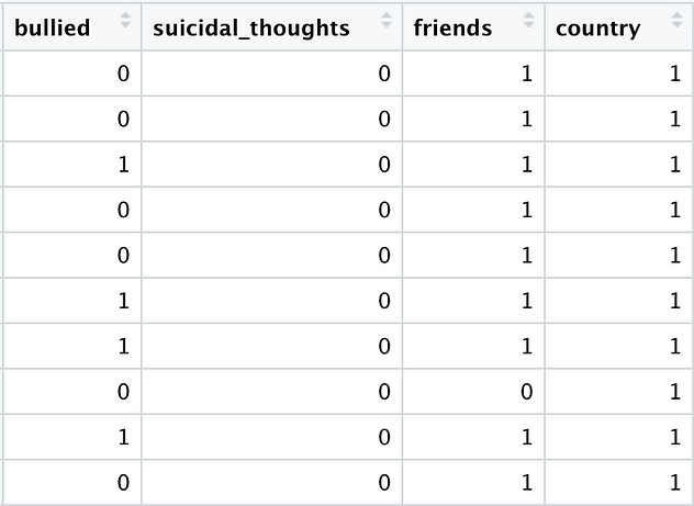
Our cleaned data frame now looks like this:
Let’s fit our models:
- Simple Logistic Regression
With the exception of variable names and the data specified, the glm() code remains identical to that used with the Fragile Families study data.
glm(formula = suicidal_thoughts ~ bullied + friends,
    family = binomial, data = survey) %>%
  broom::tidy()
Unsurprisingly, whether or not a child has friends and whether or not a child is bullied are both significant predictors of the presence of suicidal thoughts in this sample.

2. Generalized Estimating Equations
gee = gee(suicidal_thoughts ~ bullied + friends, data = survey,
          id = country, family = binomial,
          corstr = "exchangeable")summary(gee)
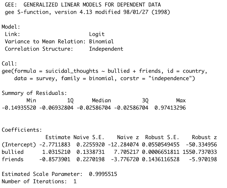
One of the reasons that I particularly like the gee() function is that the naive standard error and Z-test statistics are actually included in the output (naive meaning that these values are produced by regression where clustering is not accounted for — you’ll see that these are exactly the same as those produced by the glm() function above). You’ll notice drastic changes in the standard errors and Z-test statistics produced using GEE (“Robust”), although both of our predictors remain significant. It appears that accounting for within-country correlation has allowed for much lower standard errors to be used.
3. Multilevel Modeling***
***Note: As noted above, models are for demonstration purposes only and are not necessarily valid. In this case, we would want more groups than two for our MLM model (meaning data from additional countries). If you are really only using two groups with MLM models, you should consider a small sample size correction.
Finally, we try MLM with the survey dataset. The code is exactly the same as that used with the Fragile Families study data, but with the new formula, grouping variable, and dataset specified.
mlm = summary(glmer(formula =
                    suicidal_thoughts ~ bullied + friends +
                    (1 | country),
                    data = survey, family = binomial))mlm$coefficients
Again, beta estimates and standard error estimates are now adjusted slightly from those produced using glm(). Z- and p-values associated with the “bullied” and “friends” variables are slightly smaller, although bullying and having friends remain significant predictors of suicidal thoughts.

Which model is best for these examples?
Data from Princeton University’s Fragile Families & Child Wellbeing Study would be best represented using GEE. This is due to the maximum cluster size of 2 observations, the fact that individual families have multiple data points over time, and the fact that we were more interested in accounting for grouping in the standard error estimates than actually assessing differences between families.
Multilevel modeling is most appropriate for data from the Global School-Based Student Health Survey (GSHS) because the data were collected cross-sectionally and can be divided into two large clusters. Additionally, the output could be further explored to determine both within- and between-group variances, and we might be interested in relationships both within and across countries.
How you account for violations of the independent observations assumption will depend on the structure of your data and your general knowledge of the data collection process, as well as whether or not you consider the correlation to be an annoyance to adjust for or something meaningful to explore.
In conclusion, regression is flexible and certain regression models can handle correlated data. However, it is always important to check the assumptions of a given technique and to make sure that your analytic strategy is appropriate for your data.


