This is Newt! And he has a binary classification problem

This is Newt. Living in a mythical world, Newt aspires to become the best dragon trainer. But a dragon only accepts someone as his forever owner if his owner is the first creature it sees right after hatching. A bit like love at the first sight, coincidental yet so precious!
That’s why Newt has been searching high and low for hatchable dragon eggs. Unfortunately, a hatchable egg is really difficult to come by.
What’s more? Distinguishing between hatchable eggs and unhatchable ones is super tedious. Newt often spends hours after hours trying to examine dragon eggs having different shapes, coming from various species with distinct appearances together with god only knows how many more environmental factors that could make an egg less likely to hatch.
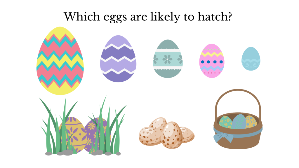
Poor Newt can’t afford to hatch all the eggs he found because his incubator only has limited slots. Thus, he has to find a better way before driving himself nuts. After all, he wants to be a skillfull dragon trainer, not a professional egg analyst.
On his way to the forest to search for dragon eggs, Newt bumped into Max, an avid tech-lover. Max shared his ideas on how to teach a computer to identify hatchable eggs based on egg images and the related environmental readings where the egg was found.
And boom! That’s how Newt got started with machine learning. Specifically, Newt needs to train a classification model to identify hatchable eggs from unhatchable ones.
Spoilt for choices. Which one to choose?
When it comes to classification models, Newt is spoilt for choices: Logistic regression, XGBoost Classifier, Random Forest Classifier, AdaBoost Classifer and so on.
Even if Newt can shortlist to a single model, he also has to choose the best one among different variations as he tunes different hyperparameters (a.k.a. hyperparameter optimisation) or utilises different features (a.k.a. feature engineering).
Simply put, among different model types, fine-tuned hyperparameters and features, Newt needs a quantifiable way to pick the best classification model. And that’s what evaluation metrics are for.
In the next sections, we will explore:
- Confusion matrix: the basis of all metrics
- Accuracy, precision, recall, F1 Score
- ROC curve and ROC AUC
Confusion matrix: The basis of all metrics
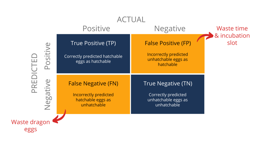
A confusion matrix just a way to record how many times the classification model correctly or incorrectly classify things into the corresponding buckets.
For example, the model initially classified 10 eggs as hatchable. However, out of those 10 eggs, only 6 are hatchable while the remaining 4 are unhatchable. In this case, the True Positive (TP) is 6 while the False Positive (FP) is 4.
Similarly, if the model classified 10 eggs as unhatchable. Out of which, 7 is actually unhatchable while the remaining 3 can hatch. We say the True Negative (TN) is 7 while False Negative (FN) is 3.
You might also have already heard about type I and type II error in statistical hypothesis testing. Simply put, False Positive is a Type I error while False Negative is a Type II error.
The most important takeaway here is that False Positive and False Negative imply two different impacts.
For instance, Newt would be wasting time and limited slots in his incubator to care for too many unhatchable eggs if the model results in too many False Positive. On the flip side, if there are too many False Negative, Newt would be wasting a lot of hatchable dragon eggs because he won’t incubate those that the model has wrongly classified as unhatchable.
Accuracy, recall, precision and F1 score
The absolute count across 4 quadrants of the confusion matrix can make it challenging for an average Newt to compare between different models. Therefore, people often summarise the confusion matrix into the below metrics: accuracy, recall, precision and F1 score.
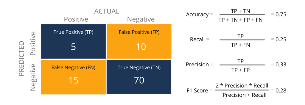
In a typical ML project, these counting and calculations are already automated. Hence, you can easily retrieve these predefined values with scikit-learn.metrics, tf.keras.metrics and so on.
However, not understanding how the count is distributed across 4 quadrants of the confusion matrix and blindly relying on a single metrics could be a risky move. Below is an overview of each metric and where it falls short.
Accuracy
Accuracy is probably the most intuitive metric to understand because it focuses on how often the prediction aligns with reality (i.e. True Positive and True Negative). So a model with 0.99 accuracy seems to be way better than our current model with 0.75 accuracy, right?
Not so fast!
High accuracy can be misleading because it does not illustrate how True Positive and True Negative distributes. For example, I can simply classify all eggs as unhatchable to obtain the below confusion matrix together with a model boasting 99% accuracy.
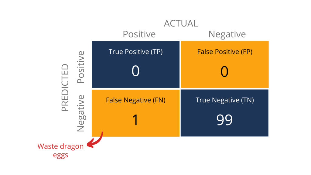
Pretty sure Newt will scream his lungs out because the model is clearly useless in helping him find hatchable eggs since all are labelled as unhatchable anyway.
Even if predictions are spread out between hatchable and unhatchable, there is still another issue. Accuracy doesn’t tell Newt what types of errors the classification model is making.
Remember how I said earlier that different errors mean different impacts for Newt? Ignoring False Positive and False Negative completely means Newt could end up with a model that wastes his precious time, incubation slots or dragon eggs.
Luckily, precision and recall are two metrics that consider False Positive and False Negative. Say hello to precision and recall!
Precision & Recall
If hatchable eggs are what Newt focuses on, precision aims to answer one question: Consider all eggs that are classified as hatchable by the model (TP+ FP), how many of them actually can be hatched into dragons (TP)?
On the other hand, recall (also known as sensitivity) focuses on a very different angle of the problem: Among all eggs that can be hatched into dragons (TP + FN), how many of them can be spotted by the model (TP)?
Both precision and recall range from 0 to 1. As a general rule of thumb, the closer to 1, the better the model is. Unfortunately, you can’t have the best of both worlds because increasing precision would cause recall to drop and vice versa. The image below illustrates this precision-recall trade-off.
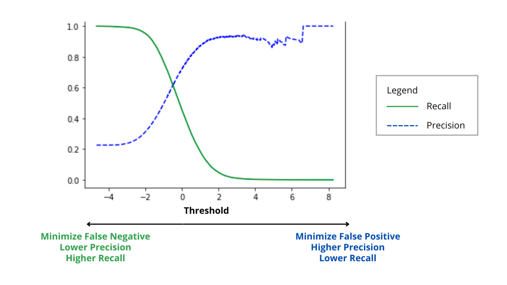
Here is a simple way to imagine what’s going on between precision and recall.
- If we classify all eggs as hatchable (i.e. all positive), then FN = 0 while FP increases significantly. Consequently, recall is now 1 while precision would drop closer to 0.
- If we classify all eggs as unhatchable (i.e. all negative), then FP = 0 whereas FN rises drastically. This means precision is now 1, whereas recall would decline closer to 0.
Given the tradeoffs between precision and recall, how should Newt choose the most optimal classification model? Well, Newt would have to ask himself whether reducing False Negative is more or less important than minimising False Positive.
Remember I said earlier that False Positive and False Negative means different impacts? Specifically, Newt would have to make a conscious choice between wasting hatchable dragon eggs (reducing False Negative and favours high precision) or wasting time and incubation slots (minimising False Positive and favours high recall).
Since life is precious and dragon eggs are so difficult to come by, a dedicated dragon lover like Newt could be more willing to choose a model having high recall with low precision.
F1 Score
But what if our scenario indicates both precision and recall are essential? Well, that’s when F1 Score comes into the picture.
F1 Score is often called the harmonic mean of the model’s precision and recall. Similar to recall and precision, the closer it is to 1, the better the model is.
This metric is often useful for evaluating classification models when neither precision nor recall is clearly more important.
In real-life datasets, the data can be imbalanced, with one classification appears much more often than another. For example, fraud cases could be rarer than normal transactions. F1 Score would also come in handy to evaluate classification models for such imbalanced datasets.
And this also concludes our section about 4 basic metrics based on the almighty confusion matrix. In the next section, let’s take it up a notch with Receiver Operating Characteristic (ROC) curve.
ROC curve and ROC AUC
ROC curve
I find it somewhat interesting to cover what ROC stands for. So here is how the story went! During World War II, the US army wanted to improve the ability to detect enemy objects on battlefields. Among all initiatives, the ROC curve was developed to measure the ability of a radar receiver operator to correctly identify Japanese aircraft based on radar signal.
Fast forward to modern days, the ROC curve has been used in various industries such as medicine, radiology, meteorology as well as machine learning. Nevertheless, people still refer to its original name: Receiver Operating Characteristic (ROC) curve.
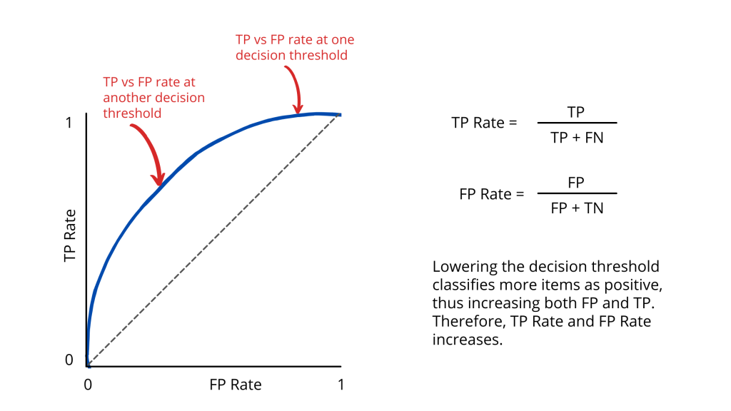
Let’s take a look at the ROC curve shown above. I know the name and the look of the graph may sound a bit intimidating. But at its core, below are 4 key points you need to know.
Firstly, an ROC curve is a graph showing the performance of a classification model across all decision thresholds.
- Generally, the closer the ROC curve is to the upper left corner, the better performance the model has.
- At the bare minimum, the ROC curve of a model has to be above the black dotted line (which shows the model at least performs better than a random guess).
Secondly, the performance of the model is measured by 2 parameters:
- True Positive (TP) rate: a.k.a. recall
- False Positive (FP) rate: a.k.a. probability of a false alarm
Thirdly, a decision threshold represents a value to convert a predicted probability into a class label. For example, let say Newt choose a threshold of 0.6 for hatchable eggs. If the model calculates the probability of an egg being hatchable is greater than or equal to 0.6, that egg will be classified as hatchable. Vice versa, if the probability is below 0.6, that egg is classified as unhatchable.
Finally, as we choose a lower threshold, more items will be classified as positive. This leads to more TP and FP, thus boosting the TP rate and FP rate accordingly.
Apart from visualising model performance, the ROC curve also illustrates a crucial point: Determining the ideal threshold requires trade-offs between TP rate and FP rate in a way that makes sense for your business objectives.
In this case, if Newt chooses too high a threshold, he might be wasting a lot of dragon eggs because most are wrongly classified as unhatchable. On the flip side, a low threshold could see him spending months incubating so many eggs but never reap any rewards.
ROC AUC
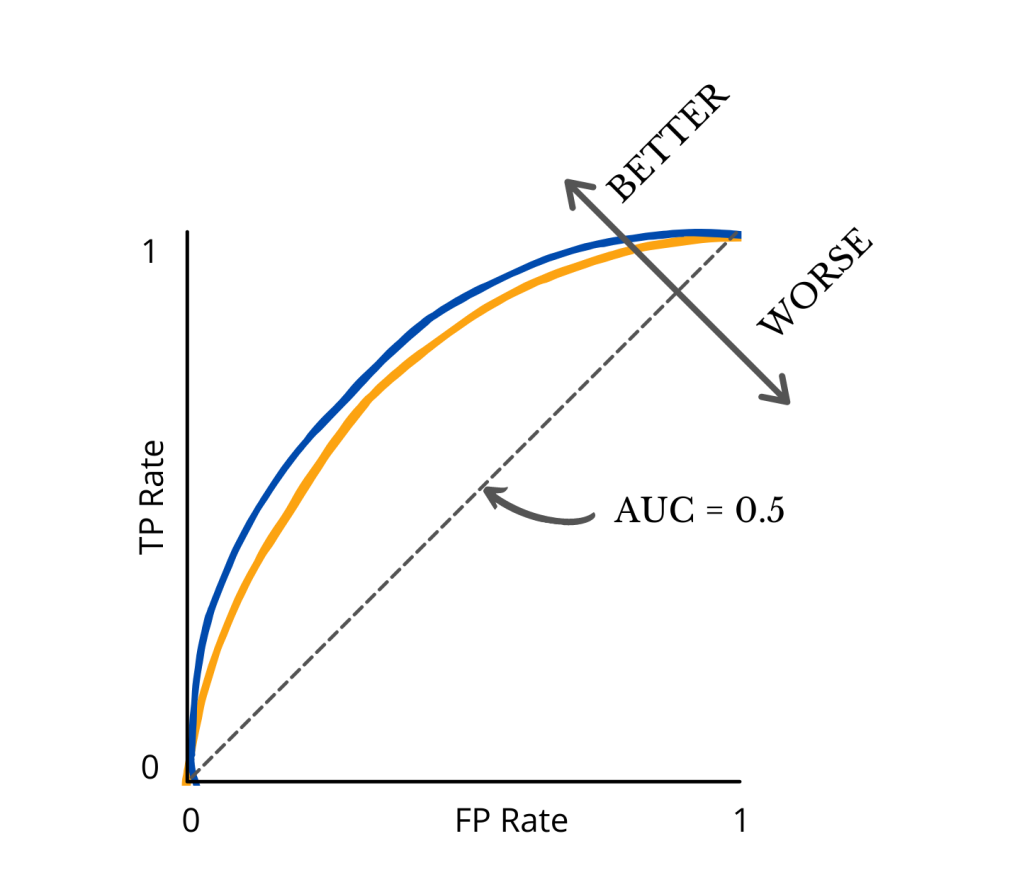
Looking at the picture above, it’s relatively easy to see the blue curve is above the yellow curve, indicating better performance. But what if we have a few more curves representing different models?
Well, the diagram could become too cluttered for anyone to decipher which is which. What’s more? For many people, it could be much simpler to look at a numeric value instead of comparing the curves.
That’s where AUC, which stands for Area Under the Curve, would come in handy. Ranging from 0 to 1, AUC measures the entire two-dimensional area underneath the entire ROC curve.
Without getting too nerdy on the mathematics, here is what you need to know: the higher the AUC value, the better the model performs at classification. At the very least, a model’s AUC has to be greater than 0.5 since it has to perform better than the random guess. Else, why should we waste time with machine learning anyway?
Parting Thoughts
So there you have it! No more confusion about what confusion matrix is and which evaluation metrics you should focus on for your next binary classification challenge. I can’t stress enough how important it is to pick the right metrics that make the most sense to your business objectives. Otherwise, you could end up choosing a model that appears to be the best, yet landing you in hot water shortly after.
That’s all I have for this blog post. Let’s say bye to Newt for now and wish him luck on his quest to become the best dragon trainer in the world!
Thank you for reading. Have feedback on how I can do better or just wanna chat? Let me know in the comments or find me on LinkedIn. Have a good one, ladies and gents!


