One of the most common misconceptions in Machine Learning is that ML Engineers get a CSV dataset and they spend the majority of the time optimizing the hyperparameters of a model.
If you work in the industry, you know that’s far from the truth. ML Engineers spend most of the time planning how to construct the training set that resembles real-world data distribution for a certain problem.
When you’ve managed to construct such training set, just add a few well-crafted features and the Machine Learning model won’t have a hard time finding the decision boundary.
In this article, we’re going to go through 8 Machine Learning tips that will help you to train a model with fewer screw-ups. These tips are most useful when you need to construct the training set, e.g. you didn’t get it from Kaggle.
At the end of the article, I also share a link to the Jupyter Notebook template, which you can incorporate into your Machine Learning workflow.
Dataset sample

It’s easier to learn with examples. Let’s create a sample dataset with random features.
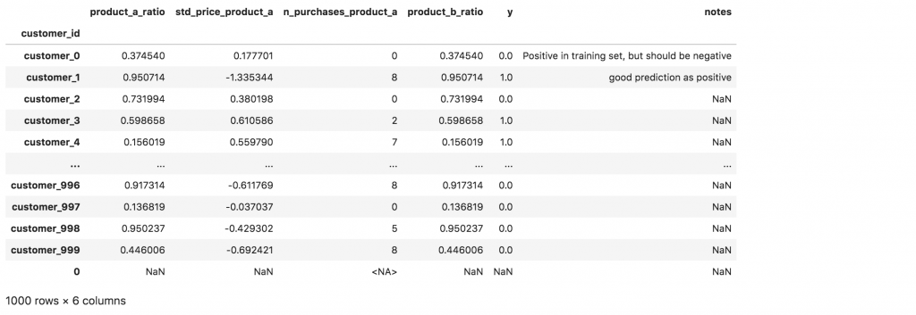
One row represents a customer with his features and a binary target variable. customer_id is an index in the DataFrame.
np.random.seed(42)n = 1000
df = pd.DataFrame(
    {
        "customer_id": ["customer_%d" % i for i in range(n)],
        "product_a_ratio": np.random.random_sample(n),
        "std_price_product_a": np.random.normal(0, 1, n),
        "n_purchases_product_a": np.random.randint(0, 10, n),
    }
)
df.loc[100, "std_price_product_a"] = pd.NA
df["product_b_ratio"] = df["product_a_ratio"]
df["y"] = np.random.randint(0, 2, n)
df.set_index("customer_id", inplace=True)df.head()

1. Check the target

Despite being obvious that no positive customer is also marked as a negative, it does happen in the real world and it’s worthwhile to check it.
assert (
    len(set(df[df.y == 0].index).intersection(df[df.y == 1])) == 0
), "Positive customers have intersection with negative customers"
I use the assert statement above in a Jupyter Notebook, which breaks execution if there is a mistake in the training set. So when I construct a new training set and use the Jupyter command: “Restart kernel and run all cells”, I can be sure that the trainset has the required properties.
When doing Exploratory Data Analysis (EDA), we need to aware that real-world datasets have mistakes in unexpected places. One of the goals of EDA is to discover them.
2. Check duplicates

How do the duplicates come into the training set?
Many times with joins in SQL databases!
E.g. you join an SQL table with another table by customer_id key. If any of those tables have multiples entries for a customer_id, it will create duplicates.
How can we make sure there aren’t any duplicates in our training set?
We can use an assert statement that will break execution in case a duplicated customer_id appears:
assert len(df[df.index.duplicated()]) == 0, "There are duplicates in trainset"
3. Check missing values

In my experience, missing values appear for two reasons:
- real missing values — the customer doesn’t have an entry for a certain feature,
- mistakes in a dataset — we didn’t map the NULL to the default value when constructing the training set, because we didn’t expect it.
In the latter case, we can simply fix the query and map the NULL value. For real missing values, we need to know how our model handles them.
For example, LightGBM supports missing values by default and we can set the desired behavior.
LightGBM uses NA (NaN) to represent missing values by default. Change it to use zero by setting zero_as_missing=true. When zero_as_missing=false (default), the unshown values in sparse matrices (and LightSVM) are treated as zeros. When zero_as_missing=true, NA and zeros (including unshown values in sparse matrices (and LightSVM)) are treated as missing.
Let’s check if our dataset contains missing values.
for col in df.columns:
    assert df[df[col].isnull()].shape[0] == 0, "%s col has %d missing values" % (col, df[df[col].isnull()].shape[0])

std_price_product_a column has a single missing value. Let’s remove the entry and rerun the check.
df = df[df['std_price_product_a'].notnull()].copy()for col in df.columns:
    assert df[df[col].isnull()].shape[0] == 0, "%s col has %d missing values" % (col, df[df[col].isnull()].shape[0])
By now, we see that these checks can be very useful. We didn’t spend a second on debugging! These checks notify us right away about the unexpected values in the dataset.
When a missing value is expected for a certain feature, we can whitelist it so the check won’t break execution next time.
4. Check feature scales

When working on feature engineering, we define certain features on a 0–1 scale or some other scale. It’s worthwhile to check if a feature in between desired boundaries.
In this example, we only check if features are on a scale between 0 and 1, but I would suggest you add more checks that are appropriate for your dataset.
features_on_0_1_scale = [
    'product_a_ratio',
    'product_b_ratio',
    'y',
]for col in features_on_0_1_scale:
    assert df[col].min() >= 0 and df[col].max() <= 1, "%s is not on 0 - 1 scale" % col
5. Check feature types

Before you start with training the model, I suggest you manually set the data type for every feature. At first, it might feel redundant, but you will thank me later.
We can set the feature types in a for loop:
feature_types = {
    "product_a_ratio": "float64",
    "std_price_product_a": "float64",
    "n_purchases_product_a": "int64",
    "product_b_ratio": "float64",
    "y": "int64",
}for feature, dtype in feature_types.items():
    df.loc[:, feature] = df[feature].astype(dtype)
Why is this useful? What happens to the integer data type when we add a missing value?
The column data type changes from integer to the object data type. When we convert it to the numpy array it has floats instead of integers. The classifier could misinterpret ordinal or categorical features as continuous features.
Let’s look at an example below:
df.n_purchases_product_a.values[:10]# output
array([0, 8, 0, 2, 7, 2, 3, 7, 0, 5])# add NA to first row
df.loc[0, "n_purchases_product_a"] = pd.NA
df.n_purchases_product_a[:10].values# output
array([0.0, 8.0, 0.0, 2.0, 7.0, 2.0, 3.0, 7.0, 0.0, 5.0], dtype=object)
6. Unique features
It’s a well-established practice in Machine Learning to define features in a list that we use in the model.
It’s worthwhile to check if a certain feature goes into the model more than once. It seems trivial but you can mistakenly duplicate features when coding and rerunning the Jupyter Notebook for X-th time.
features = [
    "product_a_ratio",
    "std_price_product_a",
    "n_purchases_product_a",
    "product_b_ratio",
]assert len(set(features)) == len(features), "Features names are not unique"
I would suggest you also list the features that you don’t use in the model. That way you can spot a feature that should be in the model but it is not.
set(df.columns) - set(features)# Output{'y'}
7. Check correlations

Checking the correlation between the features (and target) is essential when modeling.
Linear Regression is a well-known algorithm that has problems with multicollinearity — when your model includes multiple features that are similar to each other.
Highly correlated features are also problematic with models that don’t have a problem with multicollinearity, like Random Forest or Boosting. Eg. the model divides feature importance between correlated feature A and feature B, which makes feature importance misleading.
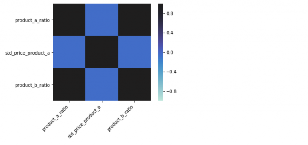
Let’s plot the correlation matrix and try to spot highly correlated features:
corr = df[features].corr()fig, ax = plt.subplots()
ax = sns.heatmap(corr, vmin=-1, vmax=1, center=1, square=True)
ax.set_xticklabels(ax.get_xticklabels(), rotation=45, horizontalalignment="right");

In the correlation matrix above, we can observe that product_a_ratio and product_b_ratio are highly correlated.
We need to be careful when removing correlated features as they can still add information despite high correlation.
In our example, features have a Pearson Correlation (PC) equal to 1.0, so we can safely remove one of them. But if the PC would be 0.9 then we could reduce the overall accuracy of the model by removing such a feature.
A good practice is also to add a comment, with a reason why we excluded the feature.
features = [
    "product_a_ratio",
    "std_price_product_a",
    "n_purchases_product_a",
    #    "product_b_ratio", # feature has pearson correlation 1.0 with product_a_ratio
]
8. Write notes

After you’ve trained the model and checked the metrics, the next step is to do a sanity check with a few samples that the model classified with confidence (customers classified with probability 0 or 1).
I usually review:
- top 5 positive predictions that are marked as positives in the training set,
- top 5 negative predictions that are marked as positives in the training set,
- top 5 positive predictions that are marked as negatives in the training set.
This requires some manual work. When retraining the model, many times those top 5 predictions change. After the X-th change, it is not clear, if you’ve already reviewed the sample or not.
To help you remember that you’ve already reviewed a customer, add a notes column to your DataFrame and write a short note to each sample that you review:
df.loc['customer_0', "notes"] = "Positive in training set, but should be negative"
df.loc['customer_1', "notes"] = "good prediction as positive"
df

Conclusion

While I was working as a Software Engineer, I found tests essential to quality software development. Tests (when well written) guarantee that the software works with given input arguments.
The tips that I’m sharing here guarantee that the dataset has the desired properties. This template can be thought of as a sequence of tests before training the model.
The template drastically reduces redundant sanity checks. There are fewer “What did I screw up again” moments.
You can download the Jupyter notebook template here.


