Convolutional Neural Networks for Beginners – Practical Guide with Python and Keras

This is the 6^th post of a series of 6 posts. You can read Post 1, Post 2, Post 3, Post 4, and Post 5 in case you missed them.

At this point, we are ready to deal with another type of neural networks, the so-called convolutional neuronal networks, widely used in computer vision tasks. These networks are composed of an input layer, an output layer and several hidden layers, some of which are convolutional, hence its name.

In this post we will present a specific case that we will follow step by step to understand the basic concepts of this type of networks. Specifically, together with the reader, we will program a convolutional neural network to solve the same MNIST digit recognition problem seen above.

Introduction to convolutional neural networks

A convolutional neuronal network (with the acronyms CNNs or ConvNets) is a concrete case of Deep Learning neural networks, which were already used at the end of the 90s but which in recent years have become enormously popular when achieving very impressive results in the recognition of image, deeply impacting the area of computer vision.

The convolutional neural networks are very similar to the neural networks of the previous posts in the series: they are formed by neurons that have parameters in the form of weights and biases that can be learned. But a differential feature of the CNN is that they make the explicit assumption that the entries are images, which allows us to encode certain properties in the architecture to recognize specific elements in the images.

To get an intuitive idea of how these neural networks work, let’s think about how we recognize things. For example, if we see a face, we recognize it because it has ears, eyes, a nose, hair, etc. Then, to decide if something is a face, we do it as if we had some mental boxes of verification of the characteristics that we are marking. Sometimes a face may not have an ear because it is covered by hair, but we also classify it with a certain probability as face because we see the eyes, nose and mouth. Actually, we can see it as a classifier equivalent to the one presented in the post “Basic concepts of neural networks”, which predicts a probability that the input image is a face or no face.

But in reality, we must first know what an ear or a nose is like to know if they are in an image; that is, we must previously identify lines, edges, textures or shapes that are similar to those containing the ears or noses we have seen before. And this is what the layers of a convolutional neuronal network are entrusted to do.

But identifying these elements is not enough to be able to say that something is a face. We also must be able to identify how the parts of a face meet each other, relative sizes, etc.; otherwise, the face would not resemble what we are used to. Visually, an intuitive idea of what layers learn is often presented with this example from an article by Andrew Ng’s group.

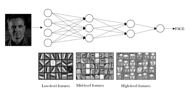
(source)

The idea that we want to give with this visual example is that, in reality, in a convolutional neural network each layer is learning different levels of abstraction. The reader can imagine that, with networks with many layers, it is possible to identify more complex structures in the input data.

Basic components of a convolutional neural network neuronal

Now that we have an intuitive vision of how convolutional neural networks classify an image, we will present an example of recognition of MNIST digits and from it we will introduce the two layers that define convolutional networks that can be expressed as groups of specialized neurons in two operations: convolution and pooling.

The convolution operation

The fundamental difference between a densely connected layer and a specialized layer in the convolution operation, which we will call the convolutional layer, is that the dense layer learns global patterns in its global input space, while the convolutional layers learn local patterns in small windows of two dimensions.

In an intuitive way, we could say that the main purpose of a convolutional layer is to detect features or visual features in images such as edges, lines, color drops, etc. This is a very interesting property because, once it has learned a characteristic at a specific point in the image, it can recognize it later in any part of it. Instead, in a densely connected neural network it has to learn the pattern again if it appears in a new location of the image.

Another important feature is that convolutional layers can learn spatial hierarchies of patterns by preserving spatial relationships. For example, a first convolutional layer can learn basic elements such as edges, and a second convolutional layer can learn patterns composed of basic elements learned in the previous layer. And so on until it learns very complex patterns. This allows convolutional neural networks to efficiently learn increasingly complex and abstract visual concepts.

In general, the convolutions layers operate on 3D tensors, called feature maps, with two spatial axes of height and width, as well as a channel axis also called depth. For an RGB color image, the dimension of the depth axis is 3, because the image has three channels: red, green and blue. For a black and white image, such as the MNIST digits, the depth axis dimension is 1 (gray level).

In the case of MNIST, as input to our neural network we can think of a space of two-dimensional neurons 28×28 (height = 28, width = 28, depth = 1). A first layer of hidden neurons connected to the neurons of the input layer that we have discussed will perform the convolutional operations that we have just described. But as we have explained, not all input neurons are connected with all the neurons of this first level of hidden neurons, as in the case of densely connected neural networks; it is only done by small localized areas of the space of input neurons that store the pixels of the image.

The explained, visually, could be represented as:

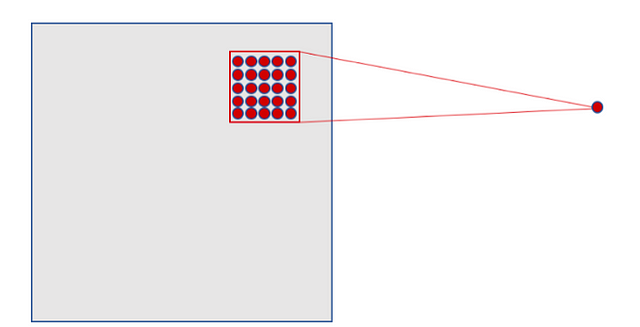
(source)

In the case of our previous example, each neuron of our hidden layer will be connected to a small region of 5×5 neurons (i.e. 25 neurons) of the input layer (28×28). Intuitively, we can think of a 5×5 size window that slides along the entire 28×28 neuron layer of input that contains the image. For each position of the window there is a neuron in the hidden layer that processes this information.

Visually, we start with the window in the top left corner of the image, and this gives the necessary information to the first neuron of the hidden layer. Then, we slide the window one position to the right to “connect” the 5×5 neurons of the input layer included in this window with the second neuron of the hidden layer. And so, successively, we go through the entire space of the input layer, from left to right and top to bottom.

Analyzing a little bit the concrete case we have proposed, we note that, if we have an input of 28×28 pixels and a window of 5×5, this defines a space of 24×24 neurons in the first hidden layer because we can only move the window 23 neurons to the right and 23 neurons to the bottom before hitting the right (or bottom) border of the input image.

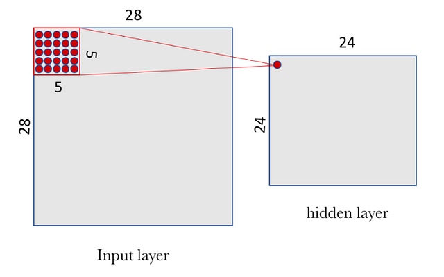
(source)

We would like to point out to the reader that the assumption we have made is that the window moves forward 1 pixel away, both horizontally and vertically when a new row starts. Therefore, in each step, the new window overlaps the previous one except in this line of pixels that we have advanced. But, as we will see in the next section, in convolutional neural networks, different lengths of advance steps can be used (the parameter called stride). In convolutional neural networks you can also apply a technique of filling zeros around the margin of the image to improve the sweep that is done with the sliding window. The parameter to define this technique is called “padding”, which we will also present in more detail in the next section, with which you can specify the size of this padding.

In our case of study, and following the formalism previously presented, to “connect” each neuron of the hidden layer with the 25 corresponding neurons of the input layer we will use a bias value b and a W-weights matrix of size 5×5 that we will call filter (or kernel). The value of each point of the hidden layer corresponds to the scalar product between the filter and the handful of 25 neurons (5×5) of the input layer.

However, the particular and very important thing about convolutional networks is that we use the same filter (the same W matrix of weights and the same b bias) for all the neurons in the hidden layer: in our case for the 24×24 neurons (576 neurons in total) of the first layer. The reader can see in this particular case that this sharing drastically reduces the number of parameters that a neural network would have if we did not do it: it goes from 14,400 parameters that would have to be adjusted (5×5 × 24×24) to 25 (5×5) parameters plus biases b.

This shared W matrix together with the b bias, which we have already said we call a filter in this context of convolutional networks, is similar to the filters we use to retouch images, which in our case are used to look for local characteristics in small groups of entries. I recommend looking at the examples found in the GIMP image editor manual to get a visual and very intuitive idea of how a convolution process works.

But a filter defined by a matrix W and a bias b only allows detecting a specific characteristic in an image; therefore, in order to perform image recognition, it is proposed to use several filters at the same time, one for each characteristic that we want to detect. That is why a complete convolutional layer in a convolutional neuronal network includes several filters.

A usual way to visually represent this convolutional layer is shown in the following figure, where the level of hidden layers is composed of several filters. In our example we propose 32 filters, where each filter is defined with a W matrix of 5×5 and a bias b.

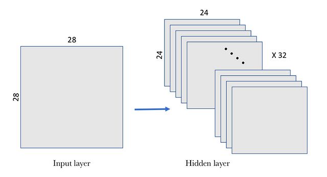
(source)

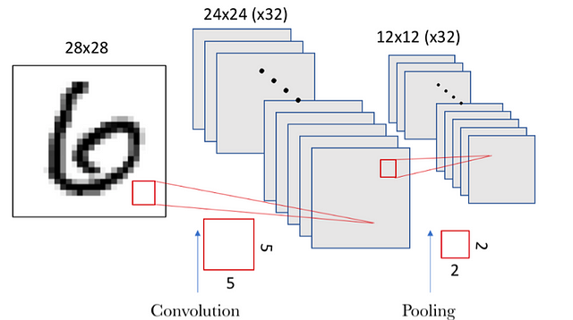
In this example, the first convolutional layer receives a size input tensor (28, 28, 1) and generates a size output (24, 24, 32), a 3D tensor containing the 32 outputs of 24×24 pixel result of computing the 32 filters on the input.

The pooling operation

In addition to the convolutional layers that we have just described, convolutional neural networks accompany the convolution layer with pooling layers, which are usually applied immediately after the convolutional layers. A first approach to understand what these layers are for is to see that the pooling layers simplify the information collected by the convolutional layer and create a condensed version of the information contained in them.

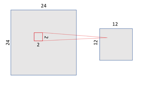
In our MNIST example, we are going to choose a 2×2 window of the convolutional layer and we are going to synthesize the information in a point in the pooling layer. Visually, it can be expressed as follows:

(source)

There are several ways to condense the information, but a usual one, which we will use in our example, is known as max-pooling, which as a value keeps the maximum value of those that were in the 2×2 input window in our case. In this case we divide by 4 the size of the output of the pooling layer, leaving an image of 12×12.

Average-pooling can also be used instead of max-pooling, where each group of entry points is transformed into the average value of the group of points instead of its maximum value. But in general, max-pooling tends to work better than alternative solutions.

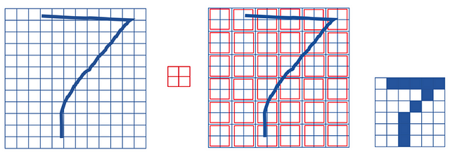
It is interesting to note that with the transformation of pooling we maintain the spatial relationship. To see it visually, take the following example of a 12×12 matrix where we have represented a “7” (Let’s imagine that the pixels where we pass over contain 1 and the rest 0; we have not added it to the drawing to simplify it). If we apply a max-pooling operation with a 2×2 window (we represent it in the central matrix that divides the space in a mosaic with regions of the size of the window), we obtain a 6×6 matrix where an equivalent representation of 7 is maintained (in the figure on the right where the zeros are marked in white and the points with value 1 in black):

(source)

As mentioned above, the convolutional layer hosts more than one filter and, therefore, as we apply the max-pooling to each of them separately, the pooling layer will contain as many pooling filters as there are convolutional filters:

(source)

The result is, since we had a space of 24×24 neurons in each convolutional filter, after doing the pooling we have 12×12 neurons which corresponds to the 12×12 regions (of size 2×2 each region) that appear when dividing the filter space.

Implementation of a basic model in Keras

Let’s see how this example of convolutional neuronal network can be programmed using Keras. As we have said, there are several values to be specified in order to parameterize the convolution and pooling stages. In our case, we will use a simplified model with a stride of 1 in each dimension (size of the step with which the window slides) and a padding of 0 (filling with zeros around the image). Both hyperparameters will be presented below. The pooling will be a max-pooling as described above with a 2×2 window.

Basic architecture of a convolutional neuronal network

Let’s move on to implement our first convolutional neuronal network, which will consist of a convolution followed by a max-pooling. In our case, we will have 32 filters using a 5×5 window for the convolutional layer and a 2×2 window for the pooling layer. We will use the ReLU activation function. In this case, we are configuring a convolutional neural network to process an input tensor of size (28, 28, 1), which is the size of the MNIST images (the third parameter is the color channel which in our case is depth 1), and we specify it by means of the value of the argument input_shape = (28, 28,1) in our first layer:

The number of parameters of the conv2D layer corresponds to the weight matrix W of 5×5 and a b bias for each of the filters is 832 parameters (32 × (25 + 1)). Max-pooling does not require parameters since it is a mathematical operation to find the maximum.

A simple model

And in order to build a “deep” neural network, we can stack several layers like the one built in the previous section. To show the reader how to do it in our example, we will create a second group of layers that will have 64 filters with a 5×5 window in the convolutional layer and a 2×2 window in the pooling layer. In this case, the number of input channels will take the value of the 32 features that we have obtained from the previous layer, although, as we have seen previously, it is not necessary to specify it because Keras deduces it:

 

If the architecture of the model is shown with the summary() method, we can see:

 

 

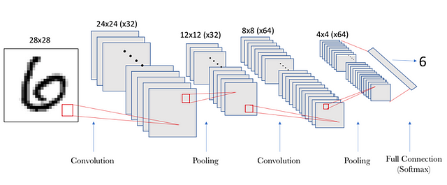
In this case, the size of the resulting second convolution layer is 8×8 since we now start from an input space of 12×12×32 and a sliding window of 5×5, taking into account that it has a stride of 1. The number of parameters 51,264 corresponds to the fact that the second layer will have 64 filters (as we have specified in the argument), with 801 parameters each (1 corresponds to the bias, and a W matrix of 5×5 for each of the 32 entries). That means ((5 × 5×32) +1) ×64 = 51264.

The reader can see that the output of the Conv2D and MaxPooling2D layers is a 3D form tensor (height, width, channels). The width and height dimensions tend to be reduced as we enter the hidden layers of the neural network. The number of kernels is controlled through the first argument passed to the Conv2D layer (usually size 32 or 64).

The next step, now that we have 64 4×4 filters, is to add a densely connected layer, which will serve to feed a final layer of softmax like the one introduced in a previous post to do the classification:

model.add(layers.Dense(10, activation=’softmax’))

In this example, we have to adjust the tensors to the input of the dense layer like the softmax, which is a 1D tensor, while the output of the previous one is a 3D tensor. That’s why we have to first flatten the 3D tensor to one of 1D. Our output (4,4,64) must be flattened to a vector of (1024) before applying the Softmax.

In this case, the number of parameters of the softmax layer is 10 × 1024 + 10, with an output of a vector of 10 as in the example in the previous post:

With the summary() method, we can see this information about the parameters of each layer and shape of the output tensors of each layer:

 

 

Observing this summary, it is easily appreciated that in the convolutional layers is where more memory is required and, therefore, more computation to store the data. In contrast, in the densely connected layer of softmax, little memory space is needed but, in comparison, the model requires numerous parameters which must be learned. It is important to be aware of the sizes of the data and the parameters because, when we have models based on convolutional neural networks, they have many layers, as we will see later, and these values can shoot exponentially.

A more visual representation of the above information is shown in the following figure, where we see a graphic representation of the shape of the tensors that are passed between layers and their connections:

(source)

Training and evaluation of the model

Once the neural network model is defined, we are ready to train the model, that is, adjust the parameters of all the convolutional layers. From here, to know how well our model does, we must do the same as we did in the Keras example of previous post “Deep Learning for Beginners: Practical Guide with Python and Keras”. For this reason, and to avoid repetitions, we will reuse the code already presented above:

As in the previous cases, the code can be found in the GitHub (source code on GitHub) of the book and it can be verified that this code offers an accuracy of approximately 97%.

If the reader has executed the code in a computer with only a CPU, it will have been noticed that, this time, the training of the network has taken a lot longer than the previous example, even with only 5 epochs. Can you imagine how long a network of many more layers, epochs or images could take? From here, as we already discussed in the introduction of the book, we need to train neuronal networks for real cases with more computing resources, such as GPUs.

The arguments of the fit method

The reader will have noticed that in this example we have not separated a part of the data for the validation of the model as we indicated in a previous section, which would be the ones that would be passed in the validation_dataargument of the fit() method. How is it possible?

As we have seen in other cases, Keras takes many values by default, and one of them is this. Actually, if the validation_data argument is not specified, Keras uses the validation_split argument, which is an integer between 0 and 1 that specifies the fraction of the training data that should be considered as validation data (argument that we have not indicated in this example).

For example, a value of 0.2 implies that 20% of the data indicated in the Numpy arrays will be separated in the first two arguments of the fit() method and will not be included in the training, being used only to evaluate the loss or any other metric at the end of each epoch. Its default value is 0.0. That is, if none of these arguments is specified, the validation process is not performed at the end of each epoch.

Actually, it does not make much sense not to do it, because the hyperparameters that we pass as arguments to the methods are very important and precisely the use of the validation data is crucial to find its best value. But in this introductory book we have thought it convenient not to go into these details and here is the simplification.

Also, this example serves to highlight that Keras has most of the hyperparameters initialized by default, in such a way that it facilitates beginners to start in the implementation of a neural network.

Hyperparameters of the convolutional layer

The main hyperparameters of the convolutional neural networks not seen until now are: the size of the filter window, the number of filters, the stride and padding.

Size and number of filters

The size of the window (window_height × window_width) that holds information from spatially close pixels is usually 3×3 or 5×5. The number of filters that tells us the number of characteristics that we want to handle (output_depth) is usually 32 or 64. In the Conv2D layers of Keras, these hyperparameters are what we pass as arguments in this order:

Conv2D(output_depth, (window_height, window_width))

Padding

To explain the concept of padding let’s use an example. Let’s suppose an image with 5×5 pixels. If we choose a 3×3 window to perform the convolution, we see that the tensor resulting from the operation is of size 3×3. That is, it shrinks a bit: exactly two pixels for each dimension, in this case. In the following figure it is visually displayed. Suppose that the figure on the left is the 5×5 image. In it, we have numbered the pixels to make it easier to see how the 3×3 drop moves to calculate the elements of the filter. In the center, it is represented how the 3×3 window has moved through the image, 2 positions to the right and two positions to the bottom. The result of applying the convolution operation returns the filter that we have represented on the left. Each element of this filter is labeled with a letter that associates it with the content of the sliding window with which its value is calculated.

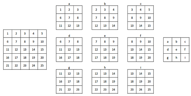
(source)

This same effect can be observed in the convolutional neuronal network example that we are creating in this post. We start with an input image of 28×28 pixels and the resulting filters are 24×24 after the first convolution layer. And in the second convolution layer, we went from a 12×12 tensioner to an 8×8 tensioner.

But sometimes we want to obtain an output image of the same dimensions as the input and we can use the hyperparameter padding in the convolutional layers for this. With padding we can add zeros around the input images before sliding the window through it. In our case in the previous figure, for the output filter to have the same size as the input image, we can add a column to the right, a column to the left, a row above and a row below to the input image of zeros. Visually it can be seen in the following figure:

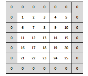
(source)

If we now slide the 3×3 window, we see that it can move 4 positions to the right and 4 positions down, generating the 25 windows that generate the filter size 5×5.

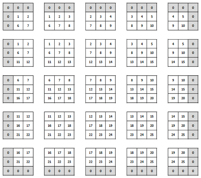
(source)

In Keras, the padding in the Conv2D layer is configured with the padding argument, which can have two values: “same”, which indicates that as many rows and columns of zeros are added as necessary so that the output has the same dimension as the entry; and “valid”, which indicates no padding (which is the default value of this argument in Keras).

Stride

Another hyperparameter that we can specify in a convolutional layer is the stride, which indicates the number of steps in which the filter window moves (in the previous example, the stride was one).

Large stride values decrease the size of the information that will be passed to the next layer. In the following figure we can see the same previous example but now with a stride value of 2:

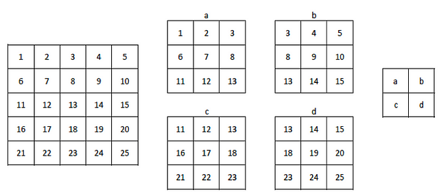
(source)

As we can see, the 5×5 image has become a smaller 2×2 filter. But in reality convolutional strides to reduce sizes are rarely used in practice; for this, the pooling operations that we have presented before are used. In Keras, the stride in the Conv2D layer is configured with the stride argument, which defaults to the strides=(1,1) value, which separately indicates the progress in the two dimensions.

source code on GitHub

Why this series of posts? The passion to teach

“Education is the most powerful weapon which you can use to change the world.” Nelson Mandela

These posts was initially designed to support my classes at the Facultat d’Informàtica de Barcelona, the faculty of Computer Science of the Universitat Politècnica de Catalunya — Barcelona Tech (UPC) with the help of my research center Barcelona Supercomputing Center (BSC-CNS).

I’m excited to share it with all my students and with the entire IT community interested in having a first contact with this technology and help them to start on their own in the programming of Deep Learning. I hope these introductory posts will help the reader interested in starting their adventure in this very interesting field.

Before finishing this series of 6 posts, let me say thanks for reading them! This fact alone makes me happy and justifies my effort in writing. Those who know me well, know that teaching (and education in general) is one of my passions and keeps me energized and motivated.