This post will show how the example of digits recognition, presented in a previous post (I strongly recommend reading it previously), is encoded with Keras to offer the reader a first practical contact with Deep Learning using this Python library.
Environment set up
Why Keras?
Keras is the recommended library for beginners, since its learning curve is very smooth compared to others, and at the moment it is one of the popular middleware to implement neural networks. Keras is a Python library that provides, in a simple way, the creation of a wide range of Deep Learning models using as backend other libraries such as TensorFlow, Theano or CNTK. It was developed and maintained by François Chollet, an engineer from Google, and his code has been released under the permissive license of MIT. Also an important thing is that Keras is included in TensorFlow as a API. Although Keras is currently included in Tensorflow package, but can also be used as a Python library. To start in the subject I consider that this second option is the most appropriate.
The code in this post is available in the form of Jupyter notebooks in the GitHub ( https://github.com/JordiTorresBCN/DEEP-LEARNING-practical-introduction-with-Keras), although this can be run as a normal program in Python if the reader so wishes.
Colaboratory environment
In this post, we will use the Colaboratory offered by Google.

It is a Google research project created to help to disseminate Machine Learning education and research. It is a Jupyter notebook environment that requires no configuration and runs completely in the Cloud allowing the use of Keras, TensorFlow and PyTorch. The most important feature that distinguishes Colab from other free cloud services is; Colab provides GPU and is totally free. Detailed information about the service can be found on the faq page.
Notebooks are stored in Google Drive and can be shared as you would do with Google Docs. This environment is free to use, which only requires a Google account. In addition, the environment allows the use of an NVIDIA K80 GPU free of charge.
When entering for the first time you will see a window like the one shown below. In this window you should select the GITHUB tab and fill in the URL field with “JordiTorresBCN” and the Repository field with “jorditorresBCN / DEEP-LEARNING-practical-introduction-with-Keras”.
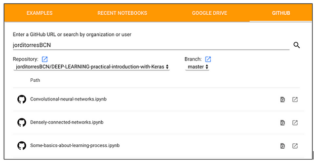
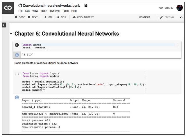
To load a notebook, click on the button that appears on their right (open notebook in new tab):
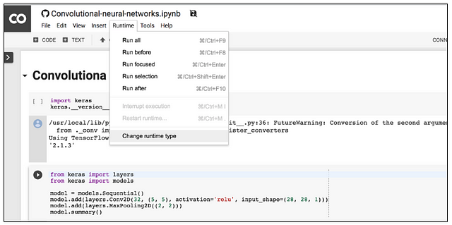
By default, Colab notebooks run on CPU. You can switch your notebook to run with GPU. In order to obtain access to one GPU we need to choose the tab Runtime and then select “Change runtime type” as shown in the following figure:
When a pop-up window appears select GPU. Ensure “Hardware accelerator” is set to GPU (the default is CPU).
A warning may appear indicating that the code is not created by Google. I hope that you trust my code and run it anyway! 😉
Afterwards, ensure that you are connected to the runtime (there is a green check next to “connected” in the menu ribbon):

Now you are able to run GitHub repo in Google Colab. Enjoy!
Data to feed a neural network
Dataset for training, validation and testing
Before presenting the implementation in Keras of the previous example, let’s review how we should distribute the available data in order to configure and evaluate the model correctly.
For the configuration and evaluation of a model in Machine Learning, and therefore Deep Learning, the available data are usually divided into three sets: training data, validation data, and test data. The training data are those used for the learning algorithm to obtain the parameters of the model with the iterative method that we have already mentioned.
If the model does not completely adapt to the input data (for example, if it presented overfitting), in this case, we would modify the value of certain hyperparameters and after training it again with the training data we would evaluate it again with the validation ones. We can make these adjustments of the hyperparameters guided by the validation data until we obtain validation results that we consider correct. If we have followed this procedure, we must be aware that, in fact, the validation data have influenced the model so that it also fits the validation data. For this reason, we always reserve a set of test data for final evaluation of the model that will only be used at the end of the whole process, when we consider that the model is already fine-tuned and we will no longer modify any of its hyperparameters.
Given the introductory nature of this post and that we will not go into detail of tuning the hyperparameters, in the examples we will ignore the validation data and only use the training and test data.
Preloaded data in Keras
In Keras the MNIST dataset is preloaded in the form of four Numpy arrays and can be obtained with the following code:
import keras
from keras.datasets import mnist
(x_train, y_train), (x_test, y_test) =mnist.load_data()
x_train and y_train contain the training set, while x_test and y_test contain the test data. The images are encoded as Numpy arrays and their corresponding labels ranging from 0 to 9. Following the strategy of the post to gradually introduce the concepts of the subject, as we have indicated, we will not see yet how to separate a part of the training data to use them as Validation data. We will only take into account the training and test data.
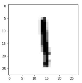
If we want to check what values we have loaded, we can choose any of the images of the MNIST set, for example image 8, and using the following Python code:
import matplotlib.pyplot as plt
plt.imshow(x_train[8], cmap=plt.cm.binary)
We get the following image:
And if we want to see its corresponding label we can do it through:
print(y_train[8])
1
That, as we see, it returns the value of “1”, as expected.
Data representation in Keras
Keras, which as we have seen uses a multidimensional array of Numpy as a basic data structure, calls this data structure a tensor. In short, we could say that a tensor has three main attributes:
- Number of axes (Rank): a tensor containing a single number will be called scalar (or a 0-dimensional tensor, or tensor 0D). An array of numbers we call vector, or tensor 1D. An array of vectors will be a matrix, or 2D tensor. If we pack this matrix in a new array, we get a 3D tensor, which we can interpret visually as a cube of numbers. By packaging a 3D tensioner in an array, we can create a 4D tensioner, and so on. In the Python Numpy library this is called the tensor’s ndim.
- Shape: it is a tuple of integers that describe how many dimensions the tensor has along each axis. In the Numpy library this attribute is called shape.
- Data type: this attribute indicates the type of data that contains the tensor, which can be for example uint8, float32, float64, etc. In the Numpy library this attribute is called dtype.
I propose that we obtain the number of axes and dimensions of the tensor train_images from our previous example:
print(x_train.ndim)
3
print(x_train.shape)
(60000, 28, 28)
And if we want to know what type of data it contains:
print(x_train.dtype)
uint8
Data normalization in Keras
These MNIST images of 28×28 pixels are represented as an array of numbers whose values range from [0, 255] of type uint8. But it is usual to scale the input values of neural networks to certain ranges. In the example of this post the input values should be scaled to values of type float32 within the interval [0, 1]. We can achieve this transformation with the following lines of code:
x_train = x_train.astype(‘float32’)
x_test = x_test.astype(‘float32’)
x_train /= 255
x_test /= 255
On the other hand, to facilitate the entry of data into our neural network (we will see that in convolutionals it is not necessary) we must make a transformation of the tensor (image) from 2 dimensions (2D) to a vector of 1 dimension (1D). That is, the matrix of 28×28 numbers can be represented by a vector (array) of 784 numbers (concatenating row by row), which is the format that accepts as input a densely connected neural network like the one we will see in this post. In Python, converting every image of the MNIST dataset to avector with 784 components can be accomplished as follows:
x_train = x_train.reshape(60000, 784)
x_test = x_test.reshape(10000, 784)
After executing these Python instructions, we can verify that x_train.shapetakes the form of (60000, 784) and x_test.shape takes the form of (10000, 784), where the first dimension indexes the image and the second indexes the pixel in each image (now the intensity of the pixel is a value between 0 and 1):
print(x_train.shape)
(60000, 784)
print(x_test.shape)
(10000, 784)
In addition to that, we have the labels for each input data (remember that in our case they are numbers between 0 and 9 that indicate which digit represents the image, that is, to which class is associated). In this example, and as we have already advanced, we will represent this label with a vector of 10 positions, where the position corresponding to the digit that represents the image contains a 1 and the remaining positions of the vector contain the value 0.
In this example we will use what is known as one-hot encoding, which we have already mentioned, which consists of transforming the labels into a vector of as many zeros as the number of different labels, and containing the value of 1 in the index that corresponds to the value of the label. Keras offers many support functions, including to_categorical to perform precisely this transformation, which we can import from keras.utils:
from keras.utils import to_categorical
To see the effect of the transformation we can see the values before and after applying to_categorical :
print(y_test[0])
7
print(y_train[0])
5
print(y_train.shape)
(60000,)
print(x_test.shape)
(10000, 784)
y_train = to_categorical(y_train, num_classes=10)
y_test = to_categorical(y_test, num_classes=10)
print(y_test[0])
[0. 0. 0. 0. 0. 0. 0. 1. 0. 0.]
print(y_train[0])
[0. 0. 0. 0. 0. 1. 0. 0. 0. 0.]
print(y_train.shape)
(60000, 10)
print(y_test.shape)
(10000, 10)
Now we have the data ready to be used in our simple model example that we are going to program in Keras in the next section.
Densely connected networks in Keras
In this section, we will present how to specify in Keras the model that we have defined in the previous sections.
Sequential class in Keras
The main data structure in Keras is the Sequential class, which allows the creation of a basic neural network. Keras also offers an API that allows implementing more complex models in the form of a graph that can have multiple inputs, multiple outputs, with arbitrary connections in between, but it is beyond the scope of this post.
The Sequential class of the Keras library is a wrapper for the sequential neural network model that Keras offers and can be created in the following way:
from keras.models import Sequential
model = Sequential()
In this case, the model in Keras is considered as a sequence of layers and each of them gradually “distills” the input data to obtain the desired output. In Keras we can find all the required types of layers that can be easily added to the model through the add() method.
Defining the model
The construction in Keras of our model to recognize the images of digits could be the following:
from keras.models import Sequential
from keras.layers.core import Dense, Activation
model = Sequential()
model.add(Dense(10, activation=’sigmoid’, input_shape=(784,)))
model.add(Dense(10, activation=’softmax’))
Here, the neural network has been defined as a sequence of two layers that are densely connected (or fully connected), meaning that all the neurons in each layer are connected to all the neurons in the next layer. Visually we could represent it in the following way:
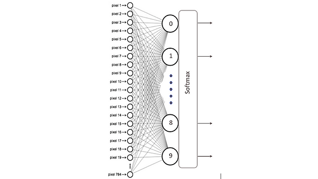
In the previous code we explicitly express in the input_shape argument of the first layer what the input data is like: a tensor that indicates that we have 784 features of the model (in fact the tensor that is being defined is (None, 784,)as we will see more ahead).
A very interesting characteristic of the Keras library is that it will automatically deduce the shape of the tensors between layers after the first one. This means that the programmer only has to establish this information for the first of them. Also, for each layer we indicate the number of nodes that it has and the activation function that we will apply in it (in this example, sigmoid).
The second layer in this example is a softmax layer of 10 neurons, which means that it will return a matrix of 10 probability values representing the 10 possible digits (in general, the output layer of a classification network will have as many neurons as classes, except in a binary classification, where only one neuron is needed). Each value will be the probability that the image of the current digit belongs to each one of them.
A very useful method that Keras provides to check the architecture of our model is summary():
model.summary()
_________________________________________________________________
Layer (type) Output Shape Param #
=================================================================
dense_1 (Dense) (None, 10) 7850
_________________________________________________________________
dense_2 (Dense) (None, 10) 110
=================================================================
Total params: 7,960
Trainable params: 7,960
Non-trainable params: 0
Later we will go into more detail with the information that returns the summary() method, because this calculation of parameters and sizes of the data that the neural network has when we start to build very large network models is very valuable. For our simple example, we see that it indicates that 7,960 parameters are required (column Param #), which correspond to 7,850 parameters to the first layer and 110 to the second.
In the first layer, for each neuron i (between 0 and 9) we require 784 parameters for the weights wij and therefore 10×784 parameters to store the weights of the 10 neurons. In addition to the 10 additional parameters for the 10 bj biases corresponding to each one of them. In the second layer, being a softmax function, it is required to connect all 10 neurons with the 10 neurons of the previous layer. Therefore 10×10 wi parameters are required and in addition 10 bj biases corresponding to each node.
The details of the arguments that we can indicate for the Dense layer can be found in the Keras manual. In our example, the most relevant ones appear. The first argument indicates the number of neurons in the layer; the following is the activation function that we will use in it. In the next post (soon 🙂 )we will discuss in more detail other possible activation functions beyond the two presented here: sigmoid and softmax.
The initialization of the weights is also often indicated as an argument of the Dense layers. The initial values must be adequate for the optimization problem to converge as quickly as possible. The various initialization options can also be found in the Keras manual.
Basic steps to implement a neural network in Keras
Next, we will present a brief description of the steps we must perform to implement a basic neural network and, in the following posts (soon), we will gradually introduce more details about each of these steps.
Configuration of the learning process
From the Sequential model, we can define the layers in a simple way with the add() method, as we have advanced in the previous section. Once we have our model defined, we can configure how its learning process will be with the compile() method, with which we can specify some properties through method arguments.
The first of these arguments is the loss function that we will use to evaluate the degree of error between calculated outputs and the desired outputs of the training data. On the other hand, we specify an optimizer that, as we will see, is the way we have to specify the optimization algorithm that allows the neural network to calculate the weights of the parameters from the input data and the defined loss function. More detail of the exact purpose of the loss function and the optimizer will be presented in the next post (soon).
And finally we must indicate the metric that we will use to monitor the learning process (and test) of our neural network. In this first example we will only consider the accuracy (fraction of images that are correctly classified). For example, in our case we can specify the following arguments in compile()method to test it on our computer:
model.compile(loss=”categorical_crossentropy”,
optimizer=”sgd”,
metrics = [‘accuracy’])
In this example we specify that the loss function is categorical_crossentropy, the optimizer used is the stocastic gradient descent (sgd) and the metric is accuracy, with which we will evaluate the percentage of correct guesses.
Model training
Once our model has been defined and the learning method configured, it is ready to be trained. For this we can train or “adjust” the model to the training data available by invoking the fit() method of the model:
model.fit(x_train, y_train, batch_size=100, epochs=5)
In the first two arguments we have indicated the data with which we will train the model in the form of Numpy arrays. The batch_size argument indicates the number of data that we will use for each update of the model parameters and with epochs we are indicating the number of times we will use all the data in the learning process. These last two arguments will be explained in much more detail in the next post (soon).
This method finds the value of the parameters of the network through the iterative training algorithm that we mentioned and we will present in a bit more detail in the next post (soon). Roughly, in each iteration of this algorithm, this algorith takes training data from x_train, passes them through the neural network (with the values that their parameters have at that moment), compares the obtained result with the expected one (indicated in y_train) and calculates the loss to guide the adjustment process of the model parameters, which intuitively consists of applying the optimizer specified above in the compile() method to calculate a new value of each one of the model parameters (weights and biases)in each iteration in such a way that the loss is reduced.
This is the method that, as we will see, may take longer and Keras allows us to see its progress using the verbose argument (by default, equal to 1), in addition to indicating an estimate of how long each epoch takes:
Epoch 1/5
60000/60000 [========] — 1s 15us/step — loss: 2.1822 — acc: 0.2916
Epoch 2/5
60000/60000 [========] — 1s 12us/step — loss: 1.9180 — acc: 0.5283
Epoch 3/5
60000/60000 [========] — 1s 13us/step — loss: 1.6978 — acc: 0.5937
Epoch 4/5
60000/60000 [========] — 1s 14us/step — loss: 1.5102 — acc: 0.6537
Epoch 5/5
60000/60000 [========] — 1s 13us/step — loss: 1.3526 — acc: 0.7034
10000/10000 [========] — 0s 22us/step
This is a simple example so that the reader at the end of the post has already been able to program their first neural network but, as we will see, the fit()method allows many more arguments that have a very important impact on the learning outcome. Furthermore, this method returns a History object that we have omitted in this example. Its History.history attribute is the record of the loss values for the training data and other metrics in successive epochs, as well as other metrics for the validation data if they have been specified.
Model evaluation
At this point, the neural network has been trained and its behavior with new test data can now be evaluated using the evaluation() method. This method returns two values:
test_loss, test_acc = model.evaluate(x_test, y_test)
These values indicate how well or badly our model behaves with new data that it has never seen. These data have been stored in x_test and y_test when we have performed the mnist.load_data() and we pass them to the method as arguments. In the scope of this post we will only look at one of them, the accuracy:
print(‘Test accuracy:’, test_acc)
Test accuracy: 0.9018
The accuracy is telling us that the model we have created in this post, applied to data that the model has never seen before, classifies 90% of them correctly.
The reader should note that, in this example, to evaluate the model we have only focused on its accuracy, that is, the ratio between the correct predictions that the model has made over the total predictions regardless of what category it is. However, although in this case it is sufficient, sometimes it is necessary to delve a little more and take into account the types of correct and incorrect predictions made by the model in each of its categories.
In Machine Learning, a very useful tool for evaluating models is the confusion matrix, a table with rows and columns that count the predictions in comparison with the real values. We use this table to better understand how well the model behaves and it is very useful to show explicitly when one class is confused with another. A confusion matrix for a binary classifier like the one explained in the previous post has this structure:
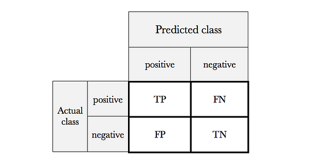
True positives (TP), true negatives (TN), false positives (FP), and false negatives (FN), are the four different possible outcomes of a single prediction for a two-class case with classes “1” (“positive”) and “0” (“negative”).
A false positive is when the outcome is incorrectly classified as positive, when it is in fact negative. A false negative is when the outcome is incorrectly classified as negative when it is in fact positive. True positives and true negatives are obviously correct classifications.
With this confusion matrix, the accuracy can be calculated by adding the values of the diagonal and dividing them by the total:
Accuracy = (TP + TN) / (TP + FP + FN + TN)
Nonetheless, the accuracy can be misleading in terms of the quality of the model because, when measuring it for the concrete model, we do not distinguish between the false positive and false negative type errors, as if both had the same importance. For example, think of a model that predicts if a mushroom is poisonous. In this case, the cost of a false negative, that is, a poisonous mushroom given for consumption could be dramatic. On the contrary, a false positive has a very different cost.
For this reason we have another metric called Sensitivity (or recall) that tells us how well the model avoids false negatives:
Sensitivity = TP / (TP + FN)
In other words, from the total of positive observations (poisonous mushrooms), how many the model detects.
From the confusion matrix, several metrics can be obtained to focus other cases as shown in this link, but it is beyond the scope of this post to enter more in detail on this topic. The convenience of using one metric or another will depend on each particular case and, in particular, the “cost” associated with each classification error of the model.
But the reader will wonder how is this confusion matrix in our classifier, where there are 10 classes instead of 2. In this case, I suggest using the Scikit-learn package to evaluate the quality of the model by calculating the confusion matrix, presented in the following figure:
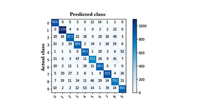
In this case, the elements of the diagonal represent the number of points in which the label predicted by the model coincides with the actual value of the label, while the other values indicate the cases in which the model has classified incorrectly. Therefore, the higher the values of the diagonal, the better the prediction will be. In this example, if the reader calculates the sum of the values of the diagonal divided by the total values of the matrix, he or she will see that it matches the accuracy that the evaluate() method has returned.
In the GitHub of the post, the reader can find the code used to calculate this confusion matrix.
Generate predictions
Finally, readers need to know how we can use the model trained in the previous section to make predictions. In our example, it consists in predict which digit represents an image. In order to do this, Keras supply the predict()method.
To test this method we can choose any element. For ease, let’s take one from the test dataset x_test. For example let’s choose the element 11 of this dataset x_test.
Before seeing the prediction, let’s see the image to be able to check ourselves if the model is making a correct prediction (before doing the previous reshape):
plt.imshow(x_test[11], cmap=plt.cm.binary)
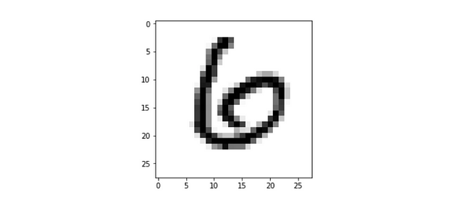
I think the reader will agree that in this case it corresponds to number 6.
Now let’s see that the predict() method of the model, executing the following code, correctly predicts the value that we have just estimated that it should predict.
predictions = model.predict(x_test)
The predict() method return a vector with the predictions for the whole dataset elements. We can know which class gives the most probability of belonging by means of the argmax function of Numpy, which returns the index of the position that contains the highest value of the vector. Specifically, for item 11:
np.argmax(predictions[11])
6
We can check it printing the vector returned by the method:
print(predictions[11])
[0.06 0.01 0.17 0.01 0.05 0.04 0.54 0. 0.11 0.02]
We see that the highest value in the vector is in the position 6. We can also verify that the result of the prediction is a vector whose sum of all its components is equal to 1, as expected. For this we can use:
np.sum(predictions[11])
1.0
So far the reader has been able to create their first model in Keras that correctly classifies the MNIST digits 90% of the time. In the next post (soon), we will present how the learning process works and several of the hyperparameters that we can use in a neural network to improve these results.
In a future post (soon) we will see how we can improve these classification results using convolutional neural networks for the same example.


