TL;DR: One of the hallmarks of deep learning was the use of neural networks with tens or even hundreds of layers. In stark contrast, most of the architectures used in graph deep learning are shallow with just a handful of layers. In this post, I raise a heretical question: does depth in graph neural network architectures bring any advantage?

This year, deep learning on graphs was crowned among the hottest topics in machine learning. Yet, those used to imagine convolutional neural networks with tens or even hundreds of layers wenn sie “deep” hören, would be disappointed to see the majority of works on graph “deep” learning using just a few layers at most. Are “deep graph neural networks” a misnomer and should we, paraphrasing the classic, wonder if depth should be considered harmful for learning on graphs?
Training deep graph neural networks is hard. Besides the standard plights observed in deep neural architectures such as vanishing gradients in back-propagation and overfitting due to a large number of parameters, there are a few problems specific to graphs. One of them is over-smoothing, the phenomenon of the node features tending to converge to the same vector and become nearly indistinguishable as the result of applying multiple graph convolutional layers [1]. This behaviour was first observed in GCN models [2,3], which act similarly to low-pass filters. Another phenomenon is a bottleneck, resulting in “over-squashing” of information from exponentially many neighbours into fixed-size vectors [4].
Significant efforts have recently been dedicated to coping with the problem of depth in graph neural networks, in hope to achieve better performance and perhaps avoid embarrassment in using the term “deep learning” when referring to graph neural networks with just two layers. Typical approaches can be split into two families. First, regularisation techniques such as edge-wise dropout (DropEdge) [5], pairwise distance normalisation between node features (PairNorm) [6], or node-wise mean and variance normalisation (NodeNorm) [7]. Second, architectural changes including various types of residual connection such as jumping knowledge [8] or affine residual connection [9]. While these techniques allow to train deep graph neural networks with tens of layers (a feat difficult or even impossible otherwise), they fail to demonstrate significant gains. Even worse, the use of deep architectures often results in decreased performance. The table below, reproduced from [7], shows a typical experimental evaluation comparing graph neural networks of different depths on a node-wise classification task:

Apparent from this table is the difficulty to disentangle the advantages brought by a deep architecture from the “tricks” necessary to train such a neural network. In fact, the NodeNorm in the above example also improves a shallow architecture with only two layers, which achieves the best performance. It is thus not clear whether a deeper graph neural network with ceteris paribus performs better.
These results are obviously in stark contrast to the conventional setting of deep learning on grid-structured data, where “ultra-deep” architectures [10,11] have brought a breakthrough in performance and are ubiquitously used today. In the following, I will try to provide directions that might help answer the provocative question raised in the title of this post. I myself do not have a clear answer yet.
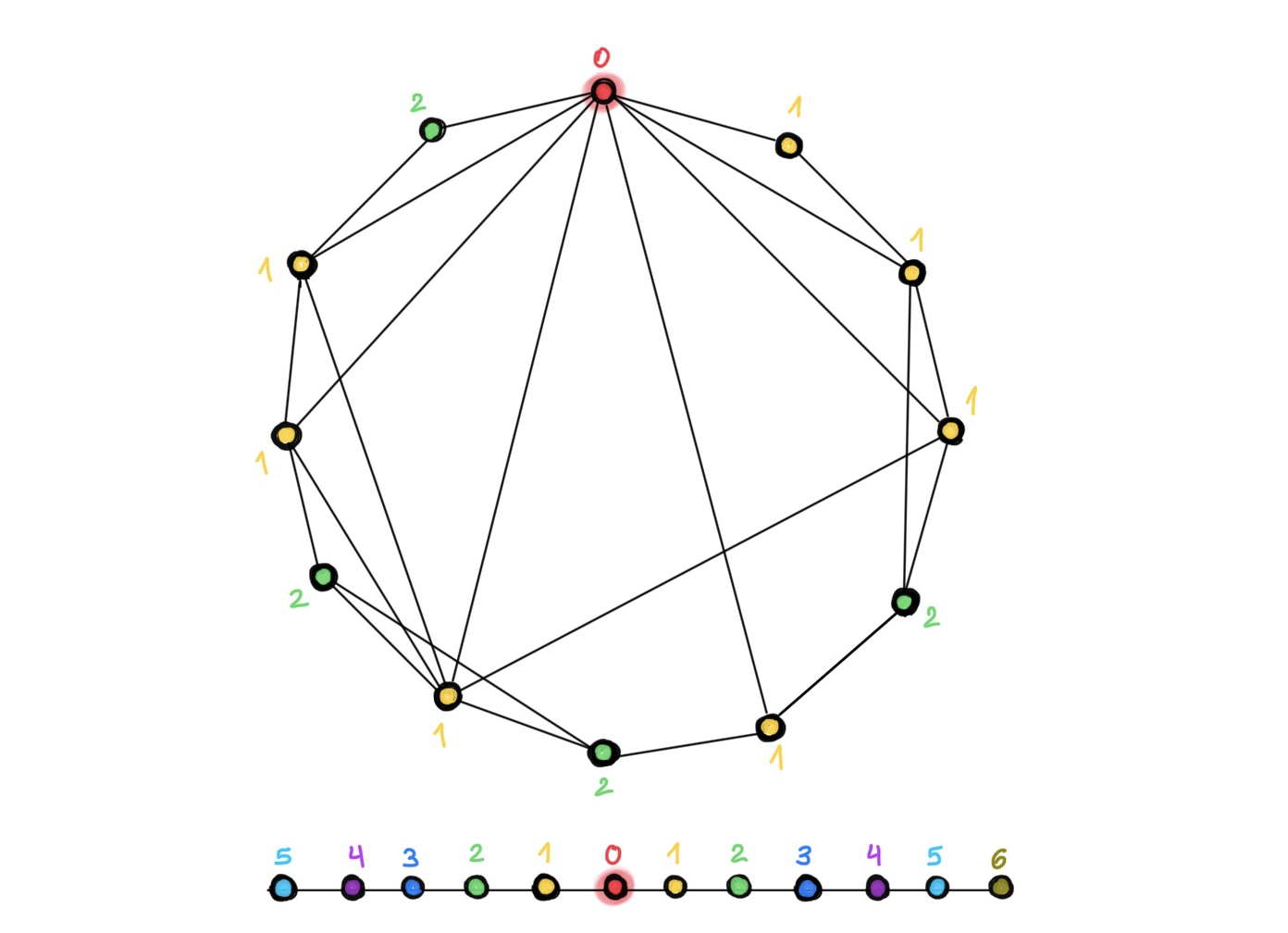
Structure of the graph. Since grids are special graphs, there certainly are examples of graphs on which depth helps. Besides grids, it appears that “geometric” graphs representing structures such as molecules, point clouds [12], or meshes [9] benefit from deep architectures as well. Why are such graphs so different from citation networks such as Cora, PubMed, or CoauthorsCS commonly used to evaluate graph neural networks? One of the differences is that the latter are similar to “small world” networks with low diameter, where one can reach any node from any other node in a few hops. As a result, the receptive field of just a few convolutional layers already covers the entire graph [13], so adding more layers does not help to reach remote nodes. In computer vision, on the other hand, the receptive field grows polynomially, and many layers are needed to produce a receptive field that captures the context of an object in the image [14].

“Do We Need Deep Graph Neural Networks?”
In small-world graphs (top), only a few hops are needed to reach any node from another one. As a result, the number of neighbours (and accordingly, the receptive field of the graph convolutional filters) grows exponentially fast. In this example, only two hops are needed in order to each any node from the red one (different colours indicate the layer in which the respective node will be reached, starting with the red one). On grids (bottom), on the other hand, the growth of the receptive field is polynomial and thus many more layers are needed to reach the same receptive field size.
Long-range vs short-range problems. A somewhat different but related distinction is whether the problem requires long or short-range information. For example, in social networks, predictions typically rely only on short-range information from the local neighbourhood of a node and do not improve by adding distant information. Such tasks can therefore be carried out by shallow GNNs. Molecular graphs, on the other hand, often require long-range information, as chemical properties of a molecule may depend on the combination of atoms at its opposite sides [15]. Deep GNNs might be needed to take advantage of these long-range interactions. However, if the structure of the graph results in the exponential growth of the receptive field, the bottleneck phenomenon can prevent the effective propagation of long-range information, explaining why deep models do not improve in performance [4].
Theoretical limitations. Besides a larger receptive field, one of the key advantages deep architectures offer in computer vision problems is their ability to compose complex features from simple ones. Visualising the features learned by CNNs from face images shows progressively more complex features starting from simple geometric primitives and ending with entire facial structures, suggesting that the legendary “grandmother neuron” is more truth than myth. It appears that such compositionality is impossible with graphs, e.g. one cannot compose triangles from edges no matter how deep the neural network is [16]. On the other hand, it was shown that the computation of some graph properties such as graph moments using message passing networks is impossible without a certain minimum depth [17]. Overall, we currently lack the understanding of which graph properties can be represented by shallow GNNs, which ones require deep models, and which ones cannot be computed at all.

Depth vs richness. As opposed to computer vision where the underlying grid is fixed, in deep learning on graphs, the structure of the graph does matter and is taken into account. It is possible to design more elaborate message passing mechanisms that account for complex higher-order information such as motifs [18] or substructure counts [19] that standard GNNs cannot discover. Instead of using deep architectures with simple 1-hop convolutions, one can opt for shallow networks with richer multi-hop filters. Our recent paper on scalable inception-like graph neural networks (SIGN) takes this idea to the extreme by using a single-layer linear graph convolutional architecture with multiple pre-computed filters. We show performance comparable to much more complex models at a fraction of their time complexity [20]. Interestingly, the computer vision community has taken the converse path: early shallow CNN architectures with large (up to 11×11) filters such as AlexNet were replaced by very deep architectures with small (typically 3×3) filters.
Evaluation. Last but not least, the predominant evaluation methodology of graph neural networks has been heavily criticised, among others by Oleksandr Shchur and colleagues from the group of Stephan Günnemann [21], who drew the attention to the pitfalls of commonly used benchmarks and showed that simple models perform on par with more complex ones if evaluated in a fair setting. Some of the phenomena we observe with deep architectures, such as performance decreasing with depth, might simply stem from overfitting on small datasets. The new Open Graph Benchmark addresses some of these issues, providing very large graphs with hard training and testing data splits. I believe that we need to do carefully designed specific experiments in order to better understand whether or when depth is useful in deep learning on graphs.
[1] More precisely, over-smoothing makes node feature vector collapse into a subspace, see K. Oono and T. Suzuki, Graph neural networks exponentially loose expressive power for node classification (2019). arXiv:1905.10947, which provides asymptotic analysis using dynamic systems formalist.
[2] Q. Li, Z. Han, X.-M. Wu, Deeper insights into graph convolutional networks for semi-supervised learning (2019). Proc. AAAI. Draws the analogy between the GCN model and Laplacian smoothing and points to the over-smoothing phenomenon.
[3] H. Nt and T. Maehara, Revisiting graph neural networks: All we have is low-pass filters (2019). arXiv:1905.09550. Uses spectral analysis on graphs to answer when GCNs perform well.
[4] U. Alon and E. Yahav, On the bottleneck of graph neural networks and its practical implications (2020). arXiv:2006.05205. Identified the over-squashing phenomenon in graph neural networks, which is similar to one observed in sequential recurrent models.
[5] Y. Rong et al. DropEdge: Towards deep graph convolutional networks on node classification (2020). In Proc. ICLR. An idea similar to DropOut where a random subset of edges is used during training.
[6] L. Zhao and L. Akoglu. PairNorm: Tackling oversmoothing in GNNs (2020). Proc. ICLR. Proposes normalising the sum of pairwise distances between node features in order to prevent them collapsing into a single point.
[7] K. Zhou et al. Effective training strategies for deep graph neural networks (2020). arXiv:2006.07107.
[8] K. Xu et al., Representation learning on graphs with jumping knowledge networks (2018). Proc. ICML 2018.
[9] S. Gong et al. Geometrically principled connections in graph neural networks (2020). Proc. CVPR.
[10] C. Szegedy et al. Going deeper with convolutions (2015). Proc. CVPR.
[11] K. He et al., Deep residual learning for image recognition (2016). Proc. CVPR.
[12] G. Li et al. DeepGCNs: Can GCNs go as deep as CNNs? (2019). Proc. ICCV. Shows the advantages of depth for geometric point-cloud data.
[13] Alon and Yahav refer to the case when a node is unable to receive information from nodes that are farther away than the number of layers as “under-reaching”. This phenomenon was first pointed out by P Barceló et al., The logical expressiveness of graph neural networks (2020). Proc. ICLR. Alon and Yahav show experimentally on the problem of chemical properties prediction in molecular graphs (using GNNs with more layers than the diameter of the graphs) that the source of poor performance is not under-reaching but over-squashing.
[14] André Araujo and co-authors have an excellent blog post about receptive fields in convolutional neural networks. As CNN models evolved in computer vision applications, from AlexNet, to VGG, ResNet, and Inception, their receptive fields increased as a natural consequence of the increased number of layers. In modern architectures, the receptive field usually covers the entire input image, i.e., the context used by each feature in the final output feature map includes all of the input pixels. Araujo et al observe a logarithmic relationship between classification accuracy and receptive field size, which suggests that large receptive fields are necessary for high-level recognition tasks, but with diminishing return.
[15] M. K. Matlock et al. Deep learning long-range information in undirected graphs with wave networks (2019). Proc. IJCNN. Observes the failure of graph neural networks to capture long-distance interactions in molecular graphs.
[16] This stems from message-passing GNN equivalence to the Weisfeiler-Lehman graph isomorphism test, see e.g. V. Arvind et al. On Weisfeiler-Leman invariance: subgraph counts and related graph properties (2018). arXiv:1811.04801 and Z. Chen et al. Can graph neural networks count substructures? (2020). arXiv:2002.04025.
[17] N. Dehmamy, A.-L. Barabási, R. Yu, Understanding the representation power of graph neural networks in learning graph topology (2019). Proc. NeurIPS. Shows that learning graph moments of certain order requires GNNs of certain depth.
[18] F. Monti, K. Otness, M. M. Bronstein, MotifNet: a motif-based Graph Convolutional Network for directed graphs (2018). arXiv:1802.01572.
[19] G. Bouritsas et al. Improving graph neural network expressivity via subgraph isomorphism counting (2020). arXiv:2006.09252.
[20] E. Rossi et al. SIGN: Scalable inception graph neural networks (2020). arXiv:2004.11198
[21] O. Shchur et al. Pitfalls of graph neural network evaluation (2018). Workshop on Relational Representation Learning. Shows that simple GNN models perform on par with more complex ones.


