Ready to learn Machine Learning? Browse Machine Learning Training and Certification courses developed by industry thought leaders and Experfy in Harvard Innovation Lab.
This is the second in a series of articles intended to make Machine Learning more approachable to those without technical training. The first article, which describes typical uses and examples of Machine Learning, can be found here.
In this installment of the series, a simple example will be used to illustrate the underlying process of learning from positive and negative examples, which is the simplest form of classification learning. I have erred on the side of simplicity to make the principles of Machine Learning accessible to all, but I should emphasize that real life use cases are rarely as simple as this.
Learning from a training set
Imagine that a company has a recruiting process which looks at many thousands of applications and separates them into two groups — those who have ‘high potential’ to receive a job with the company, and those who do not. Currently, human beings decide which group each application falls into. Imagine that we want to learn and predict which applications are considered ‘high potential’. We obtain some data from the company for a random set of prior applications, both those which were classified as high potential (positive examples) and those who were not (negative examples). We aim to find a description that is shared by all the positive examples and by none of the negative examples. Then, if a new application occurs, we can use this description to determine if the new application should be considered ‘high potential’.
Further analysis of the applications reveals that there are two main characteristics that affect whether an application could be described as ‘high potential’. The first is the College GPA of the applicant, and the second is the applicant’s performance on a test that they undertake during the application process. We therefore decide only to consider these factors in our determination of whether an application is ‘high potential’. These are our input attributes.
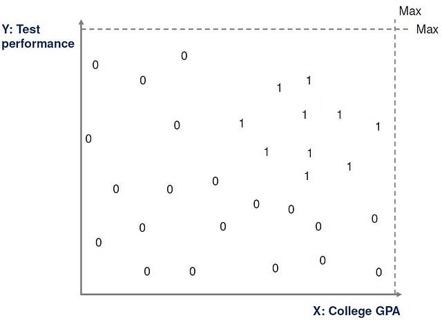
We can therefore take a subset of current applications and represent each one by two numeric values (x,y) where x is the applicant’s college GPA, and y is the applicant’s performance in the test. We can also assign each application a value of 1 if it is a positive example and 0 if it is a negative example. This is called the training set.
For this simple example, the training set can be plotted on a graph in two dimensions, with positive examples marked as a 1 and negative examples marked as a zero, as illustrated below.
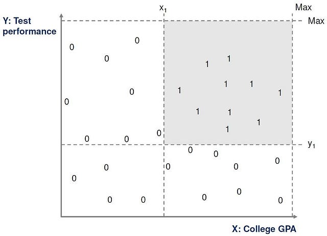
After looking at the data further, we can establish certain minimum values on the two dimensions x and y, and we can say that any ‘high potential’ application must fall above these values. That is x > x1 and y > y1 for suitable values of x1 and y1.
This then defines the set of ‘high potential’ applications as a rectangle on our chart, as shown here.
In this way, we have made the hypothesis that our class of ‘high potential’ applications is a rectangle in two-dimensional space. We now reduce the problem to finding the values of x1and y1 so that we have the closest ‘fit’ to the positive examples in our training set.
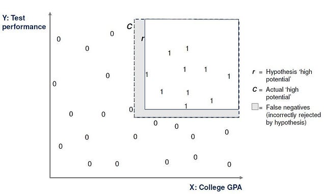
We now decide to try a specific rectangle to see how well it fits the training data. We call this rectangle r. r is a hypothesis function. We can try r on our training set and count how many instances in the training set occur where a positive example does not fall into the rectangle r. The total number of these instances is called the error of r. Our aim is to use the training set to make this error as low as possible, even to make it zero if we can.
One option is to use the most specific hypothesis. That is, to use the tightest rectangle that contains all of the positive examples and none of the negative examples. Another is to use the most general hypothesis, which is the largest rectangle that contains all the positive example and none of the negative examples.
In fact, any rectangle between the most specific and most general hypothesis will work on the specific training set we have been given.
However, our training set is just a sample list of applications, and does not include all applications. Therefore, even if our proposed rectangle r works on the training set, we cannot be sure that it would be free from error if applied to applications which are not in the training set. As a result, our hypothesis rectangle r could create errors when applied outside the training set, as indicated below.
Measuring error
When a hypothesis r is developed from a training set, and when it is then tried out on data that was not in the training set, one of four things can happen:
- True positive (TP): When r gives a positive result and it agrees with the actual data
- True negative (TN): When r gives a negative result and it agrees with the actual data
- False positive (FP): When r gives a positive result and it disagrees with the actual data
- False negative (FN): When r gives a negative result and it disagrees with the actual data. (This is the shaded area in the previous diagram)
The total error of the hypothesis function r is equal to the sum of FP and FN.
Ideally we would want this to equal zero. However…
Noise
The previous example of learning ‘high potential’ applications based on two input attributes is very simplistic. Most learning scenarios will involve hundreds or thousands of input attributes, tens of thousands of examples in the training set and will take hours, days or weeks of computer capacity to process.
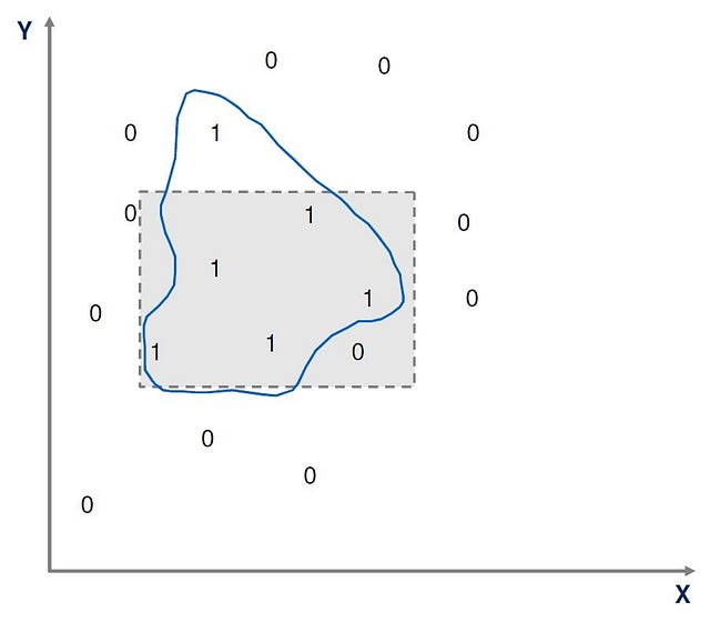
It is virtually impossible to create simple hypotheses that have zero error in these situations, due to noise. Noise is unwanted anomalies in the data that can disguise or complicate underlying relationships and weaken the learning process. The diagram below shows a dataset that may be affected by noise, and for which a simple rectangle hypothesis cannot work, and a more complex graphical hypothesis is necessary for a perfect fit.
Noise can be caused by:
- Errors or omissions in the input data
- Errors in data labeling
- Hidden attributes which are unobservable and for which no data is available, but which affect the classification.
Despite noise, data scientists will usually aim to find the simplest hypothesis possible on a training set, for example a line, rectangle or simple polynomial expression. They will be willing to accept a certain degree of training error in order to keep the hypothesis as simple as possible. Simple hypotheses are easier to construct, explain and generally require less processing power and capacity, which is an important consideration on large datasets.
Generalization, underfit and overfit
As observed above, it is necessary for a data scientist to make a hypothesis about which function best fits the data in the training set. In practical terms, this means that the data scientist is making assumptions that a certain model or algorithm is the best one to fit the training data. The learning process requires such ingoing assumptions or hypotheses, and this is called the inductive bias of the learning algorithm.
As we also observed, it is possible for a certain algorithm to fit well to a training set, but then to fail when applied to data outside the training set. Therefore, once an algorithm is established from the training set, it becomes necessary to test the algorithm against a set of data outside the training set to determine if it is an acceptable fit for new data. How well the model predicts outcomes for new data is called generalization.
If a data scientist tries to fit a hypothesis algorithm which is too simple, although it might give an acceptable error level for the training data, it may have a much larger error when new data is processed. This is called underfitting. For example, trying to fit a straight line to a relationship that is a higher order polynomial might work reasonably well on a certain training set, but will not generalize well.
Similarly, if a hypothesis function is used which is too complex, it will not generalize well — for example, if a multi-order polynomial is used in a situation where the relationship is close to linear. This is called overfitting.
Generally the success of a learning algorithm is a finely balanced trade-off between three factors:
- The amount of data in the training set
- The level of the generalization error on new data
- The complexity of the original hypothesis which was fitted to the data
Problems in any one of these can often be addressed by adjusting one of the others, but only to a degree.
The typical process of Machine Learning
Putting all of the above observations together, we can now outline the typical process used in Machine Learning. This process is designed to maximize the chances of learning success and to effectively measure the error of the algorithm.
Training: A subset of real data is provided to the data scientist. The data includes a sufficient number of positive and negative examples to allow any potential algorithm to learn. The data scientist experiments with a number of algorithms before deciding on those which best fit the training data.
Validation: A further subset of real data is provided to the data scientist with similar properties to the training data. This is called the validation set. The data scientist will run the chosen algorithms on the validation set and measure the error. The algorithm that produces the least error is considered to be the best. It is possible that even the best algorithm can overfit or underfit the data, producing a level of error which is unacceptable.
Testing: It will be important to measure the error of any learning algorithm that is considered implementable. The validation set should not be used to calculate this error as we have already used the validation set to choose the algorithm so that it has minimal error. Therefore the validation set has now effectively become a part of the training set. To obtain an accurate and reliable measure of error, a third set of data should be used, known as the test set. The algorithm is run on the test set and the error is calculated.
The typical output of a classification algorithm
The typical output of a classification algorithm can take two forms:
Discrete classifiers. A binary output (YES or NO, 1 or 0) to indicate whether the algorithm has classified the input instance as positive or negative. Using our earlier example, the algorithm would simply say that the application is ‘high potential’ or it is not. This is particularly useful if there is no expectation of human intervention in the decision making process, such as if the company has no upper or lower limit to the number of applications which could be considered ‘high potential’.
Probabilistic classifiers. A probabilistic output (a number between 0 and 1) which represents the likelihood that the input falls into the positive class. For example, the algorithm may indicate that the application has a 0.68 probability of being high potential. This is particularly useful if human intervention is to be expected in the decision making process, such as if the company has a limit to the number of applications which could be considered ‘high potential’. Note that a probabilistic output becomes a binary output as soon as a human defines a ‘cutoff’ to determine which instances fall into the positive class.

