Ready to learn Machine Learning? Browse courses like Machine Learning Foundations: Supervised Learning developed by industry thought leaders and Experfy in Harvard Innovation Lab.
In this article, we showed that how the simple sorting algorithm is at the heart of solving an important problem in computational geometry and how that relates to a widely used machine learning technique.
Machine learning (ML) is fast becoming one of most important computational techniques in the modern society. A branch of Artificial Intelligence (AI), it is being applied to everything from natural language translation and processing(think Siri or Alexa) to medicine, autonomous driving, or business strategy development. A dizzying array of clever algorithms are being developed continuously for solving ML problems to learn patterns from streams of data and build AI infrastructure.
However, sometimes it feels good to step back and analyze how some of the elementary algorithms are also doing their part in this revolution and appreciate their impact. In this article, I am going to illustrate one such non-trivial case.
Support Vector Machine
Support vector machine or SVM in short, is one of the most important machine learning techniques, developed in past few decades. Given a set of training examples, each marked as belonging to one or the other of two categories, an SVM training algorithm builds a model that assigns new examples to one category or the other, making it a non-probabilistic binarylinear classifier. It is widely used in industrial systems, text classifications, pattern recognition, biological ML applications, etc.
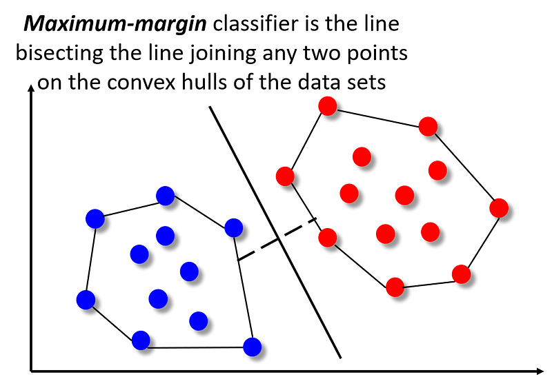
The idea is illustrated in the following picture. Main goal is to classify the points in the 2-dimensional plane into one of two categories — red or blue. It can be done by creating a classifier boundary (by running a classification algorithm and learning from the labeled data) between the two sets of points. Some of the possible classifiers are shown in the figure. All of them will classify the data points correctly but not all of them have the same ‘margin’ (i.e. distance) from the sets of data points which are closest to the boundary. It can be shown that only one of them maximizes this ‘margin’ between the set of blue and red points. That unique classifier is shown by the solid line whereas the other classifiers are shown as dotted lines. The utility of this margin maximization is that larger the distance between two classes, lower the generalization error will be for the classification of a new point.
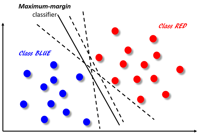
FIG 1: SVM and Maximum-margin classifier
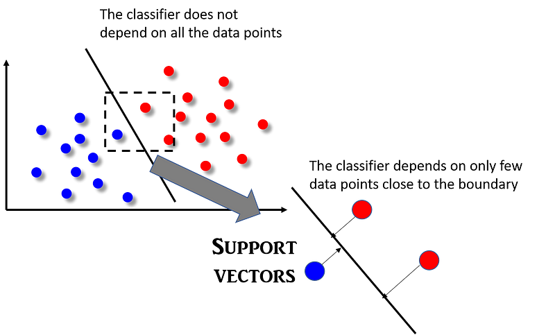
The main differentiating feature of SVM algorithm is that the classifier does not depend on all the data points (unlike say logistic regression where each data point’s features will be used in the construction of the classifier boundary function). In fact, SVM classifier depend on a very small subset of data points, those which lie closest to the boundary and whose position in the hyperplane can impact the classifier boundary line. The vectors formed by these points uniquely define the classifier function and they ‘support’ the classifier, hence the name ‘support vector machine’. This concept is shown in the following figure.
Read more on this “Idiot’s guide to support vector machines”. A nice video tutorial on SVM can be found here.
A geometric explanation of how the SVM works: Convex Hull
The formal mathematics behind the SVM algorithm is fairly complex but intuitively it can be understood by considering a special geometric construct called convex hull.
What is Convex Hull? Formally a convex hull or convex envelope or convex closure of a set X of points in the Euclidean plane or in a Euclidean space is the smallest convex set that contains X. However it is easiest to visualize using the rubber band analogy. Imagine that a rubber band is stretched about the circumference of a set of pegs (our points of interest). If the rubber band is released, it becomes wrapped around the pegs resulting in a tight border defining the original set. The resulting shape is the convex hull, and can be described by the subset of pegs that touch the border created by the rubber band. The idea is shown below.
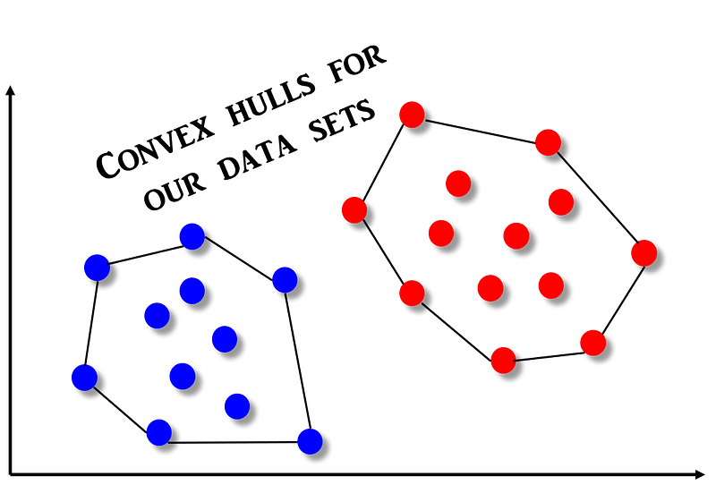
Now, it is easy to imagine that the SVM classifier is nothing but the linear separator that bisects the line joining these convex hulls exactly mid-point.
Therefore, determining the SVM classifier reduces to the problem of finding the convex hull of a set of points.
How to determine the convex hull?
Picture (an animated one) says a thousand words! Therefore, let me show the algorithm used to determine the convex hull of a set of points, in action. It is called Graham’s scan. The algorithm finds all vertices of the convex hull ordered along its boundary. It uses a stack to detect and remove concavities in the boundary efficiently.

Now, the question is how efficient this algorithm is i.e. what is the time complexity of Graham’s scan method?
It turns out that the time complexity of Graham’s scan depends on the underlying sort algorithm that it needs to employ for finding the right set of points which constitute the convex hull. But what is it sorting to begin with?
The fundamental idea of this scanning techniques comes from two properties of a convex hull,
- Can traverse the convex hull by making only counterclockwise turns
- The vertices of convex hull appear in increasing order of polar angle
with respect to point p with lowest y-coordinate.
First the points are stored in an array points. Therefore, the algorithm starts by locating a reference point. This is the point with the lowest y coordinate (in case of ties, we break the tie by selecting the point with the lowest y coordinate and the lowest x coordinate). Once we locate the reference point, we move that point to beginning of pointsby making it trade places with the first point in the array.
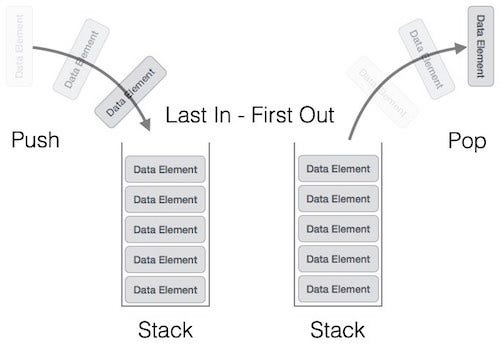
FIG: A stack data structure
Next, we sort the remaining points by their polar angle relative to the reference point. After sorting, the points with the lowest polar angle relative to the reference point will be at the beginning of the array, and the points with the largest polar angle will be at the end.
With the points properly sorted, we can now run the main loop in the algorithm. The loop makes use of a second list that will grow and shrink as we process the points in the main array. Basically, we push points, which appear in counterclockwise rotation, on to the stack and reject points (pop from the stack) if the rotation becomes clockwise. The second list starts out empty. At the end of the algorithm, the points that make up the convex boundary will appear in the list. A stack data structure is used for this purpose.
Pseudocode
# Three points are a counter-clockwise turn if ccw > 0, clockwise if
# ccw < 0, and colinear if ccw = 0 because ccw is a determinant that #gives twice the signed area of the triangle formed by p1, p2, and #p3.
function ccw(p1, p2, p3):
return (p2.x – p1.x)*(p3.y – p1.y) – (p2.y – p1.y)*(p3.x – p1.x)
let N be number of points
let points[N] be the array of points
swap points[0] with the point with the lowest y-coordinate
# This is the most time-consuming step
sort points by polar angle with points[0]
let stack = NULL
push points[0] to stack
push points[1] to stack
push points[2] to stack
for i = 3 to N:
while ccw(next_to_top(stack), top(stack), points[i]) <= 0:
pop stack
push points[i] to stack
end
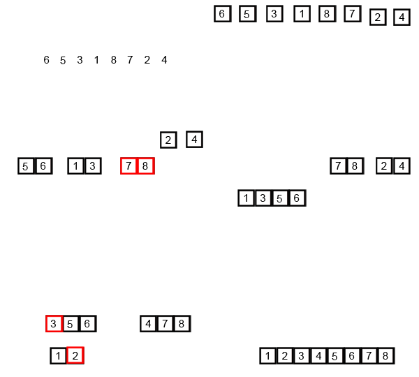
So, the time complexity of Graham’s scan depends on the efficiency of the sort algorithm. Any general purpose sort technique can be used but there is a big difference between using a O(n#k8SjZc9Dxk2) and a O(n.log(n)) algorithm (as illustrated in the following animation).
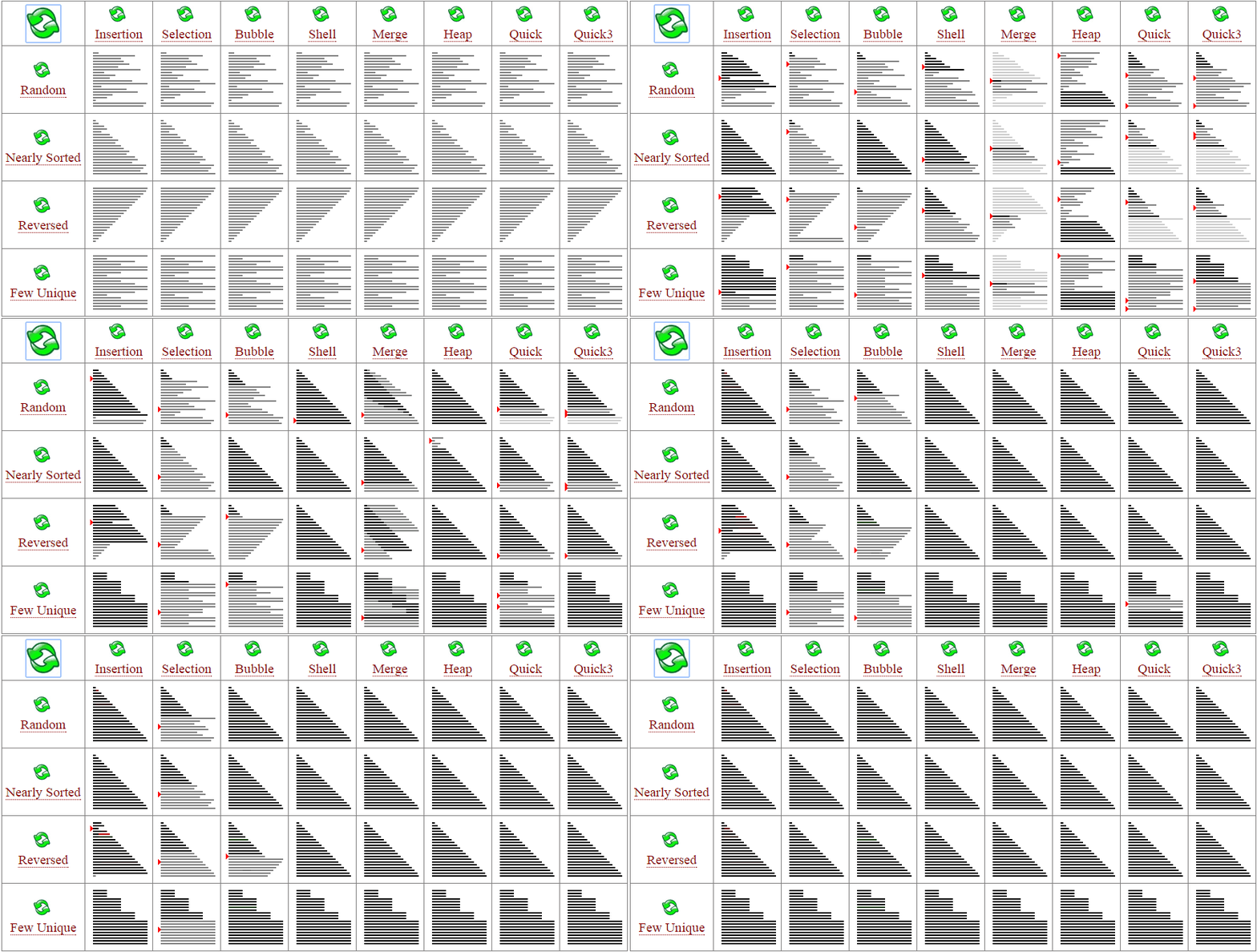
FIG: Animations of various sort algorithms
Summary
In this article, we showed that how the simple sorting algorithm is at the heart of solving an important problem in computational geometry and how that relates to a widely used machine learning technique. Although there are many discrete optimization based algorithms to solve the SVM problem, this approach demonstrates the importance of using fundamentally efficient algorithms at the core to build complex learning model for AI.


