Choosing a small, representative dataset from a large population can improve model training reliability
In machine learning, we often need to train a model with a very large dataset of thousands or even millions of records. The higher the size of a dataset, the higher its statistical significance and the information it carries, but we rarely ask ourselves: is such a huge dataset really useful? Or we could reach a satisfying result with a smaller, much more manageable one? Selecting a reasonably small dataset carrying the good amount of information can really make us save time and money.
Let’s make a simple mental experiment. Imagine that we are in a library and want to learn Dante Alighieri’s Divina Commedia word by word.
We have two options:
- Grab the first edition we find and start studying from it
- Grab as many editions as possible and study from all of them
Machine learning is the same thing. We have a model that learns something and, exactly like us, it needs some time. What we want is the minimum amount of information that is required to learn properly from the phenomenon, without wasting our time. Information redundancy doesn’t contain any business value for us.
But how can we be sure that our edition isn’t corrupted or incomplete? We must perform some kind of high-level comparison with the population made by the other editions. For example, we could check the number of canti and cantiche. If our book has three cantiche and each one of them has 33 canti, maybe it’s complete and we can safely learn from it.
What we are doing is learn from a sample (the single Divina Commedia edition) and check its statistical significance (the macro comparison with the other books).
The same, exact concept can be applied in machine learning. Instead of learning from a huge population of many records, we can make a sub-sampling of it keeping all the statistics intact.
Statistical framework
In order to take a small, easy to handle dataset, we must be sure we don’t lose statistical significance with respect to the population. A too small dataset won’t carry enough information to learn from, a too huge dataset can be time-consuming to analyze. So how can we choose the good compromise between size and information?
Statistically speaking, we want that our sample keeps the probability distribution of the population under a reasonable significance level. In other words, if we take a look at the histogram of the sample, it must be the same as the histogram of the population.
There are many ways to accomplish this goal. The simplest thing to do is taking a random sub-sample with uniform distribution and check if it’s significant or not. If it’s reasonably significant, we’ll keep it. If it’s not, we’ll take another sample and repeat the procedure until we get a good significance level.
Multivariate vs. multiple univariate
If we have a dataset made by N variables, it can be clustered in a N-variate histogram and so can be every sub-sample we can take from it.
This operation, although academically correct, can be really difficult to perform in reality, especially if our dataset mixes numerical and categorical variables.
That’s why I prefer a simpler approach, that usually introduces an acceptable approximation. What we are going to do is consider each variable independently from the others. If each one of the single, univariate histograms of the sample columns is comparable with the correspondent histogram of the population columns, we can assume that the sample is not biased.
The comparison between sample and population is then made this way:
- Take one variable from the sample
- Compare its probability distribution with the probability distribution of the same variable of the population
- Repeat with all the variables
Some of you could think that we are forgetting the correlation between variables. It’s not completely true, in my opinion, if we select our sample uniformly. It’s widely known that selecting a sub-sample uniformly will produce, with large numbers, the same probability distribution of the original population. Powerful resampling methods like bootstrap are built around this concept (see my previous article for more information).
Comparing sample and population
As I said before, for each variable we must compare its probability distribution on the sample with the probability distribution on the population.
The histograms of categorical variables can be compared using Pearson’s chi-square test, while the cumulative distribution functions of the numerical variables can be compared using the Kolmogorov-Smirnov test.
Both statistical tests work under the null hypothesis that the sample has the same distribution of the population. Since a sample is made by many columns and we want all of them to be significative, we can reject the null hypothesis if the p-value of at least one of the tests is lower than the usual 5% confidence level. In other words, we want every column to pass the significance test in order to accept the sample as valid.
R Example
Let’s move from theory to practice. As usual, I’ll use an example in R language. What I’m going to show you is how the statistical tests can give us a warning when sampling is not done properly.
Data simulation
Let’s simulate some (huge) data. We’ll create a data frame with 1 million records and 2 columns. The first one has 500.000 records taken from a normal distribution, while the other 500.000 records are taken from a uniform distribution. This variable is clearly biased and it will help me explain the concepts of statistical significance later.
The other field is a factor variable created by using the first 10 letters from the alphabet uniformly distributed.
Here follows the code to create such a dataset.
set.seed(100)
N = 1e6
dataset = data.frame(
# x1 variable has a bias. The first 500k values are taken
# from a normal distribution, while the remaining 500k
# are taken from a uniform distribution
x1 = c(
rnorm(N/2,0,1) ,
runif(N/2,0,1)
),
# Categorical variable made by the first 10 letters
x2 = sample(LETTERS[1:10],N,replace=TRUE)
)
Create a sample and check its significance
Now we can try to create a sample made by 10.000 records from the original dataset and check its significance.
Remember: numerical variables must be checked with the Kolmogorov-Smirnov test, while categorical variables (i.e. factors in R) need Pearson’s chi-square test.
For each test, we’ll store its p-value in a named list for the final check. If all the p-values are greater than 5%, we can say that the sample is not biased.
sample_size = 10000
set.seed(1)
idxs = sample(1:nrow(dataset),sample_size,replace=F)
subsample = dataset[idxs,]
pvalues = list()
for (col in names(dataset)) {
if (class(dataset[,col]) %in% c(“numeric”,”integer”)) {
# Numeric variable. Using Kolmogorov-Smirnov test
pvalues[[col]] = ks.test(subsample[[col]],dataset[[col]])$p.value
} else {
# Categorical variable. Using Pearson’s Chi-square test
probs = table(dataset[[col]])/nrow(dataset)
pvalues[[col]] = chisq.test(table(subsample[[col]]),p=probs)$p.value
}
}
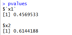
pvalues
The p-values are, then:

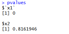
What happens if we take the first 10.000 records instead of taking them randomly? We know that the first half of the X1 variable of the dataset has a different distribution than the total, so we expect that such a sample can’t be representative of the whole population.
If we repeat the tests, these are the p-values:

Conclusions
In this article, I’ve shown you that a proper sample can be statistically significant to represent the whole population. This may help us in machine learning because a small dataset can make us train models more quickly than a larger one, carrying the same amount of information.
However, everything is strongly related to the significance level we choose. For certain kinds of problems, it can be useful to raise the confidence level or discard those variables that don’t show a suitable p-value. As usual, a proper data discovery before training can help us decide how to perform a sample correctly.
Here is the Original article.


