Unsupervised and Semi-supervised Gaussian Mixture Models (GMM)
When companies launch a new product, they usually want to find out the target customers. If they have data on customers’ purchasing history and shopping preferences, they can utilize it to predict what types of customers are more likely to purchase the new product. There are many models to solve this typical unsupervised learning problem and the Gaussian Mixture Model (GMM) is one of them.
GMM and EM
GMMs are probabilistic models that assume all the data points are generated from a mixture of several Gaussian distributions with unknown parameters. They differ from k-means clustering in that GMMs incorporate information about the center(mean) and variability(variance) of each clusters and provide posterior probabilities.
In the example mentioned earlier, we have 2 clusters: people who like the product and people who don’t. If we know which cluster each customer belongs to (the labels), we can easily estimate the parameters(mean and variance) of the clusters, or if we know the parameters for both clusters, we can predict the labels. Unfortunately, we don’t know either one. To solve this chicken and egg problem, the Expectation-Maximization Algorithm (EM) comes in handy.
EM is an iterative algorithm to find the maximum likelihood when there are latent variables. The algorithm iterates between performing an expectation (E) step, which creates a heuristic of the posterior distribution and the log-likelihood using the current estimate for the parameters, and a maximization (M) step, which computes parameters by maximizing the expected log-likelihood from the E step. The parameter-estimates from M step are then used in the next E step. In the following sections, we will delve into the math behind EM, and implement it in Python from scratch.
Mathematical Deduction
W define the known variables as x, and the unknown label as y. We make two assumptions: the prior distribution p(y) is binomial and p(x|y) in each cluster is a Gaussian .
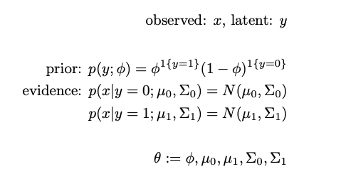
All parameters are randomly initialized. For simplicity, we use θ to represent all parameters in the following equations.

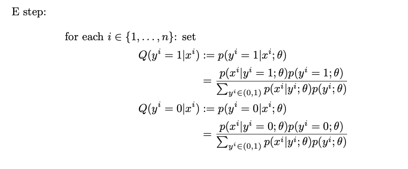
At the expectation (E) step, we calculate the heuristics of the posteriors. We call them heuristics because they are calculated with guessed parameters θ.
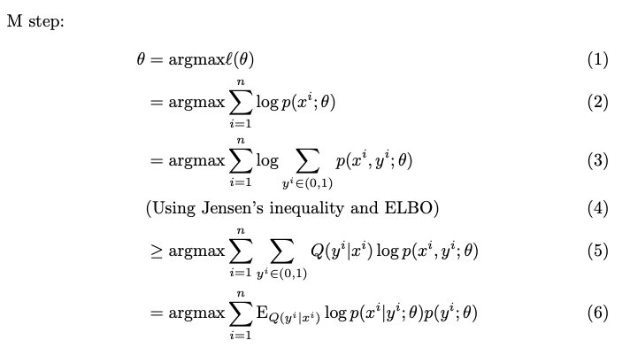
At the maximization (M) step, we find the maximizers of the log-likelihood and use them to update θ. Notice that the summation inside the logarithm in equation (3) makes the computational complexity NP-hard. To move the summation out of the logarithm, we use Jensen’s inequality to find the evidence lower bound (ELBO) which is tight only when Q(y|x) = P(y|x). If you are interested in the math details from equation (3) to equation (5), this article has decent explanation.
Luckily, there are closed-form solutions for the maximizers in GMM.
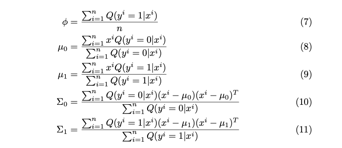
We use these updated parameters in the next iteration of E step, get the new heuristics and run M-step. What the EM algorithm does is repeat these two steps until the average log-likelihood converges.
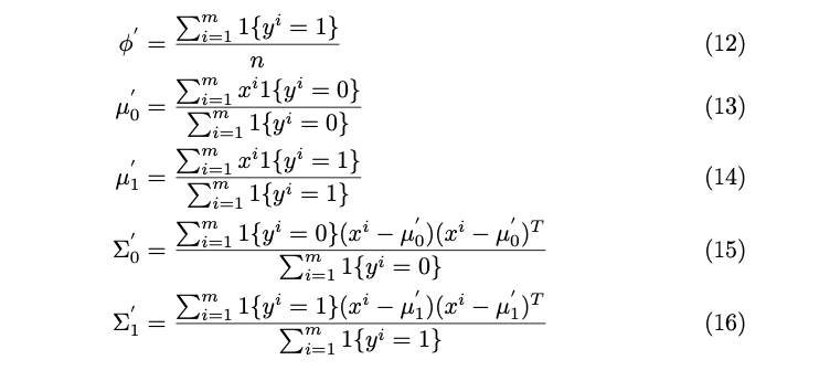
Before jumping into the code, let’s compare the above parameter solutions from EM to the direct parameter estimates when the labels are known. Did you find they are very similar? In fact, the only difference is that the EM solutions use the heuristics of posteriors Q while the direct estimates use the true labels.
Python Implementation
There are many packages including scikit-learn that offer high-level APIs to train GMMs with EM. In this section, I will demonstrate how to implement the algorithm from scratch to solve both unsupervised and semi-supervised problems. The complete code can be find here.
1. Unsupervised GMM
Let’s stick with the new product example. Using the known personal data, we have engineered 2 features x1, x2 represented by a matrix x, and our goal is to forecast whether each customer will like the product (y=1) or not (y=0).https://towardsdatascience.com/media/de0e60977c7b85502cad24a0abe46e8d
First we initialize all the unknown parameters.get_random_psd() ensures the random initialization of the covariance matrices is positive semi-definite.
https://gist.github.com/VXU1230/426921e27f0dfa6fa76aeaa95faec54f#file-initialize_random_params-py
Then we pass the initialized parameters to e_step()and calculate the heuristics Q(y=1|x) and Q(y=0|x) for every data point as well as the average log-likelihoods which we will maximize in the M step.
https://gist.github.com/VXU1230/dca3f37734759c278eaeb29a92020d80#file-e_step-py
In m_step() , the parameters are updated using the closed-form solutions in equation(7) ~ (11). Note that if there weren’t closed-form solutions, we would need to solve the optimization problem using gradient ascent and find the parameter estimates.
https://gist.github.com/VXU1230/3f6db97cce7a9c6969b83fa9c1c7d712#file-m_step-py
Now we can repeat running the two steps until the average log-likelihood converges. rum_em() returns the predicted labels, the posteriors and average log-likelihoods from all training steps.
https://gist.github.com/VXU1230/c86fc58a1d3043a6fde6f48d6ccb1f9a#file-run_em-py
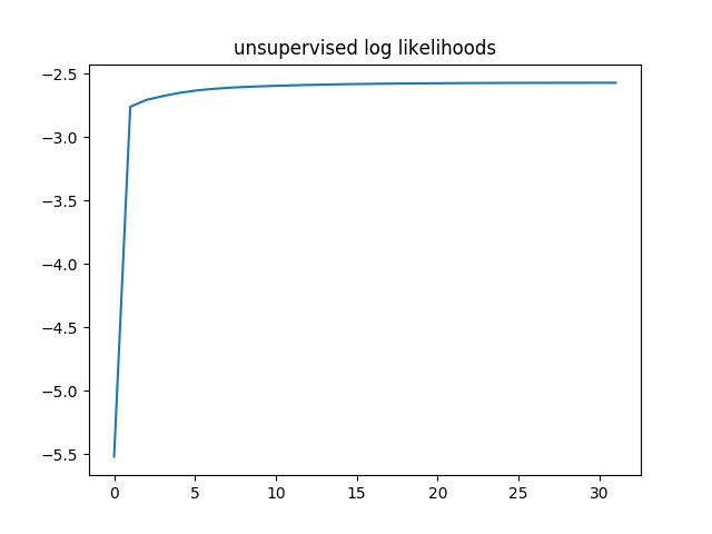
Running the unsupervised model , we see the average log-likelihoods converged in over 30 steps.
https://gist.github.com/VXU1230/ebf0771d2f9ef4635ad21eb1688dcd34#file-unsupervised-py
2. Semi-supervised GMM
In some cases, we have a small amount of labeled data. For example, we might know some customers’ preferences from surveys. Considering the potential customer base is huge, the amount of labeled data we have is insufficient for full supervised learning, yet we can learn the initial parameters from the data in a semi-supervised way.
We use the same unlabeled data as before, but we also have some labeled data this time.
https://gist.github.com/VXU1230/9b6648f5202522c6ef2756e6ede74ab2#file-load_labeled_data-py
In learn_params() , we learn the initial parameters from the labeled data by implementing equation (12) ~(16). These learned parameters are used in the first E step.
https://gist.github.com/VXU1230/77ca2a26190920d4724501453e84ba0c#file-learn_params-py
Other than the initial parameters, everything else is the same so we can reuse the functions defined earlier. Let’s train the model and plot the average log-likelihoods.
https://gist.github.com/VXU1230/33b51d76fe736bd82d67a731ad50f441#file-semi-supervised-py
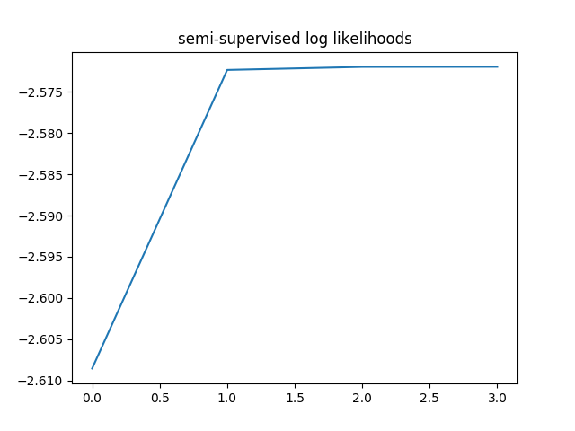
This time the average log-likelihoods converged in 4 steps, much faster than unsupervised learning.
To verify our implementation, we compare our forecasts with forecasts from the scikit-learn API. To build the model in scikit-learn, we simply call the GaussianMixture API and fit the model with our unlabeled data. Don’t forget to pass the learned parameters to the model so it has the same initialization as our semi-supervised implementation.GMM_sklearn()returns the forecasts and posteriors from scikit-learn.
https://gist.github.com/VXU1230/3e3dafedb33ed8b30689957ec356b969#file-compare_sklearn-py
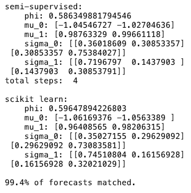
Comparing the results, we see that the learned parameters from both models are very close and 99.4% forecasts matched. In case you are curious, the minor difference is mostly caused by parameter regularization and numeric precision in matrix calculation.
That’s it! We just demystified the EM algorithm.
Conclusions
In this article, we explored how to train Gaussian Mixture Models with the Expectation-Maximization Algorithm and implemented it in Python to solve unsupervised and semi-supervised learning problems. EM is a very useful method to find the maximum likelihood when the model depends on latent variables and therefore is frequently used in machine learning.
I hope you had fun reading this article 🙂


