This article appeared in Towards Data Science
A high-level structural overview of classical Reinforcement Learning algorithms
A RL algorithm can be described as a model that indicates to an agent which set of actions it should take within a closed environment in order to to maximize a predefined overall reward. Generally speaking, the agent tries different sets of actions, evaluating the total obtained return. After many trials, the algorithm learns which actions give a greater reward and establishes a pattern of behavior. Thanks to this, it is able to tell the agent which actions to take in every condition.
Applications
Let’s see some examples of applications based on RL:
- Robotics – RL can be used for high-dimensional control problems and for various industrial applications.
- Text mining – RL, along with a text generation model, can be used to develop a system that is able to produce highly readable summaries of long texts.
- Trade execution – Major companies in the financial industry use RL algorithms to improve their trading strategy.
- Healthcare – RL is useful for medication dosing, and for the optimization of treatment for people suffering from chronic clinical trials, etc.
- Games -RL is famous for being the main algorithm used to solve different games and to achieve superhuman performances.
Actors
RL algorithms are based on Markov Decision Process (MDP). A Markov Decision Processes is a special stochastic time control process for decision making. The main actors of a RL algorithm are:
- Agent: an entity which performs actions in an environment in order to optimize a long-term reward;
- Environment: the scenario in which the agent takes decisions;
- Set of states (S): the set of all the possible states s of the environment, where the state describes the current situation of the environment;
- Set of actions (A): the set of all the possible actions a that can be performed by the agent;
- State transition model P (s_0|s , a): describes the probability that the environment state changes in s_0 when the agent performs the action a at state s, for every states s, s_0 and action a;
- Reward (r = R(s , a)): a function that indicates the immediate the real valued reward for taking action a at state s;
- Episode (rollout): it’s a sequence of states st and actions at for t that varies from 0 to a final value L (that is called horizon and can eventually be infinite); the agent starts in a given state of its environment; at each timestep t the agent observes the current state s_t ∈ S and consequently takes an action a_t ∈ A; the state evolves into a new state s_(t+1), that depends only on the state s_t and on the action a_t , according to the state transition model; the agent obtains a reward r_t; then the agent observes the new state s_(t+1)∈ S and the loop restarts;
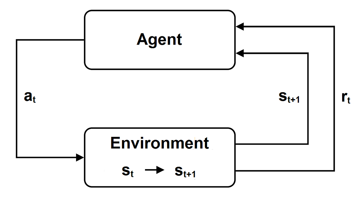
- Policy function: a policy can be deterministic (π (s)) or stochastic ((a|s)): a deterministic policy π (s) indicates the action a performed by the the agent when the environment is in the state s (a = π (s)); a stochastic policy π (a|s) is a function that describe the probability that action a is performed by the the agent when the environment is in the state s. Once that the policy is specified, the new state only depends on the policy and on the state transaction model;
- Return G_t : the total long term reward with discount obtained at the end of the episode, according to the immediate reward of the current timestep and of every following timesteps, and to the the discount factor γ < 1:

- Value function V(s): the expected long-term return at the end of the episode, starting from state s at current timestep t:

- Q-Value or Action-Value function Q(s , a): the expected long-term return at the end of the episode, starting from state s at current timestep, and performing action a;
- The Bellman equation: the theoretical core in most RL algorithms; according to it, the current value function is equal to the current reward plus itself evaluated at the next step and discounted by γ (we recall that in the equation P is the model transition model):

Optimal policy


The problem is that in most real cases the state transition model and the reward function are unknown, so it’s necessary to learn them from sampling in order to estimate the optimal action value function and the best policy. For these reasons RL algorithms are used, in order to take the actions in the environment, observe and learn the dynamics of the model, estimate the optimal value function and the optimal policy, and improve the rewards.
Exploration-exploitation dilemma

Approaches
There are 3 main possible approaches that we can use when we implement a RL algorithm:
- Value-based methods – A Value-based algorithm approximates the optimal value function, or the optimal action value function, by continuously improving their estimate. Usually the value function or the action value function are initialized randomly, then they are continuously updated until they converge. A Value-based algorithm is guaranteed to converge to the optimal values.
- Policy-based methods – A Policy-based algorithm looks for a policy such that the action performed at each state is optimal to gain maximum reward in the future. It redefines the policy at each step and computes the value function according to this new policy until the policy converges. A Policy-based method is also guaranteed to converge to the optimal policy, and often takes less iterations to converge than the value-based algorithms.
- Model-based methods – A Model-based algorithm learns a virtual model starting from the original environment, and the agent learns how to perform in the virtual model. It uses a reduced number of interactions with the real environment during the learning phase, then it builds a new model based on these interactions, uses this model to simulate the further episodes, and and get the results returned by the virtual model.
Value-based methods
Value Function Approximation

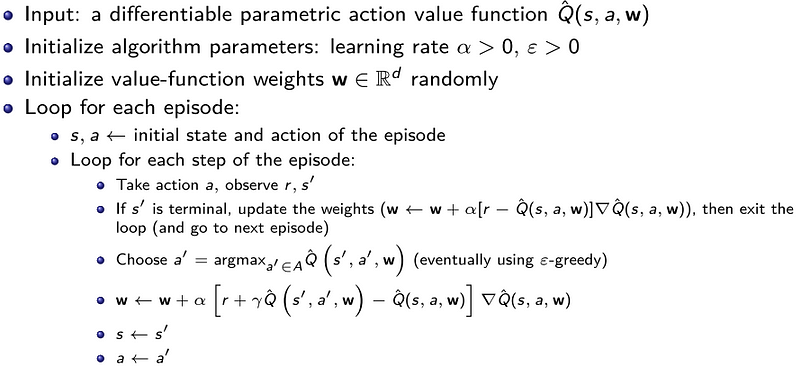
Deep Q-Networks
- Target Network – The model updates could be very unstable since the real target changes each time the model updates itself. The solution is to create a Target Network Q^(s’,a’,w’), which is a copy of the training model that is updated less frequently, for example every thousands steps (we indicate as w’ the weights of the Target Network). In every model update with the gradient descent, the Target Network is used as target in place of the model itself:

- Experience Replay – In the described algorithm several consecutive updates are performed using data from the same episode, and this can cause overfitting. To solve this, it is created an Experience Replay buffer that stores the four-tuples (s,a,r,s’) of all the different episodes, and randomly select a batch of tuples each time the model is updated. This solution has 3 advantages: reduces overfitting, increases learning speed with mini-batches, and reuses past tuples to avoid forgetting.
Fitted Q-Iteration

Consider now a temporal horizon N less than or equal to the horizon L, and denote by Q_N (s , a) the action value function over N steps defined by the application of the just defined operator H to the action value function Q_(N−1) (s , a), with

It is possible to show that this sequence of N-step action value functions Q_N (s , a) converges to the optimal action value function Q*(s , a) as N → L. Thanks to this, it’s possible to build an algorithm to approximate the optimal action value function Q*(s , a) iterating on N.
Fitted Q-Iteration algorithm:
A full implementation of Fitted Q-Iteration can be found on GitHub
(https://github.com/teopir/ifqi).
Fitted Q-Iteration algorithm:Fitted Q-Iteration algorithm:Fitted Q-Iteration algorithm:
Consider a car, modeled by a point mass, that is traveling on a hill with this form:
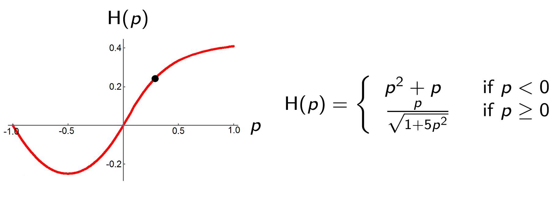
The control problem goal is to bring the car in a minimum time to the top of the hill while preventing the position p of the car to become smaller than -1 and its speed v to go outside the interval [-3 , 3]. The top of the hill is reached at position p = 1.
State space – This problem has a (continuous) state space of dimension two (the position p and the speed v of the car), and we want that the absolute value of the position is less than or equal to 1, and that the absolute value of the speed is less than or equal to 3:

Every other combination of position and speed is considered a terminal state.
Action space – The action a acts directly on the acceleration of the car and can
only assume two extreme values (full acceleration (a = 4) or full deceleration (a -4)). Hence the action space is given by the set

System dynamics – The time is discretized in timesteps of 0.1 seconds. Given the state (p, v) and the action a at timestep t, we are able to compute the state (p, v) at timestep t + 1 solving with a numeric method the two differential equations related to position and speed that describe the dynamic of the system:

Of course for our purpose it’s not important to understand the meaning of these equations, it’s important to understand that given state and action at timestep t, the state at timestep t + 1 in uniquely determined.
Reward function – The reward function r(s , a) is defined through this expression:

The reward is -1 if the position is less then -1 or if the absolute value of the speed is greater than 3 because we reached a termination state but we didn’t reach the top of the hill; the reward is 1 if the position is greater than 1 and the absolute value of the speed is less than 3 because we reached the top of the hill respecting the speed limits; otherwise the reward is 0.
Discount factor – The decay factor γ has been chosen equal to 0.95.
Initial point – At the begin the car stopped at the bottom of the hill (p , v) = (0.5, 0).
Regressor – The regressor used is an Extra Tree Regressor.
Performing the Fitted Q-Iteration for N = 1 to 50 it turns out that for N > 20 the mean squared error between action value functions Q^_N (s , a) and Q^_(N+1)(s , a) (computed on all the combinations of (p, v)) decreases quickly to 0 as N increases. For this reason the results are studied using the action state function Q^_20(s , a).
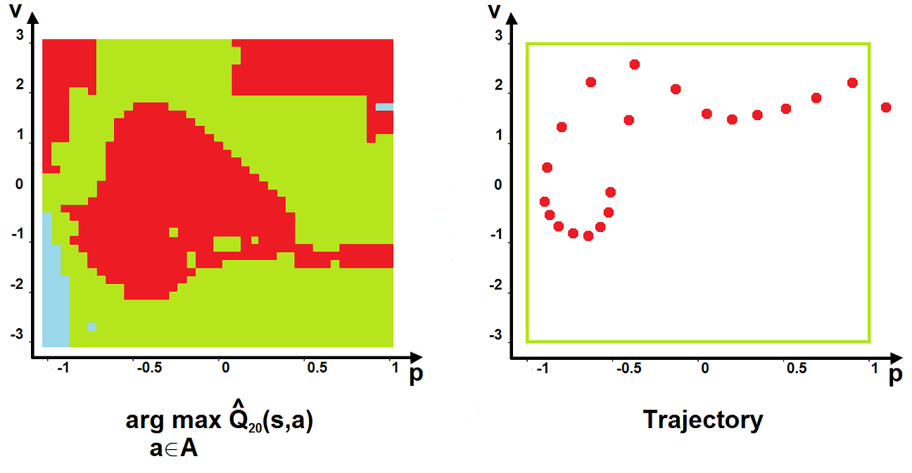
In figure on the left we can see the action chosen for every combination of
(p, v), according to the action value function Q^_20(s , a) (red area represents deceleration, green area represents acceleration, blu area means that the action values of deceleration and acceleration are equal).
The optimal trajectory according to the action value function Q^_20(s , a) is represented in the figure on the right.
Policy-valued Methods
Policy Gradient
Policy Gradient os the most classical Policy-based method. The goal of the Policy Gradient method is to find the vector of parameters θ that maximizes the value function V (s , θ) under a parametric policy π (a|s , θ).
We start considering a parametric policy π (a|s , θ) differentiable with respect to the vector of parameters θ; in particular in this case we choose a stochastic policy (in this case the method is called Stochastic Policy Gradient, however the case with a deterministic policy is very similar).
We initialize randomly the vector w and we iterate on every episode. For each timestep t we generate a sequence of triplets (s, a, r) choosing the action according the parametric policy π (a|s , θ). For every timestep in the resulting sequence we compute the total long term reward with discount G_t in function of the obtained rewards:

Then the vector of parameters θ_t is modified using a gradient update process

In the equation α > 0 is the learning rate.
It can be shown that this process converges, and the obtained process is our approximated optimal policy.
Policy Gradient algorithm:

Examples of parametric policies
The most used parametric policies are Softmax Policy and Gaussian Policy.
Softmax Policy
The Softmax Policy consists of a softmax function that converts output to a
distribution of probabilities, and is mostly used in the case discrete actions:

In this case the explicit formula for the gradient update is given by

where φ(s , a) is the feature vector related to the state and the action.
Gaussian Policy
The Gaussian Policy is used in the case of a continuous action space, and is given by the Gaussian function

where µ(s) is given by φ(s) T θ, φ(s , a) is feature vector, and σ can be fixed or parametric. Also in this case we have the explicit formula for the gradient update:

Advantages and Disadvantages of Policy Gradient
Advantages
- A Policy Gradient method is a simpler process compared with value-based
methods. - It allows the action to be continuous with respect to the state.
- It usually has better convergence properties with respect to other methods.
- It avoids the growth in the usage of memory and in the computation time when the action and state sets are large, because the goal is to learn a set of parameters whose size is much smaller than that of the set of states and the set of actions.
- It can learn stochastic policies.
- It allows the use ϵ-greedy method, so that the agent can have a probability ϵ of taking random actions.
Disadvantages
- A Policy Gradient method typically converges to a local rather than global
optimum. - It usually has high variance (that however can be reduced with some techniques).
Example of Policy Gradient application: CartPole
CartPole is a game where a pole is attached by an unactuated joint to a cart, which moves along a frictionless track. The pole starts upright.

The goal is to prevent the pole from falling over by increasing and reducing the cart’s velocity.
State space – A single state is composed of 4 elements:
- cart position
- cart velocity
- pole angle
- pole angular velocity
The game ends when the pole falls, which is when the pole angle is more than ±12°, or the cart position reaches the edge of the display.
Action space – The agent can take only 2 actions:
- move the pole to the left
- move the pole to the right
Reward – For every step taken (including the termination step), the reward is increased by 1. This is obviously because we want to achieve the greatest possible number of steps.
The problem is solved with Gradient Policy method using Softmax Policy, with discount factor γ = 0.95 and learning rate α = 0.1. For every episode a maximum number of 1000 iterations is fixed.
After about 60 epochs (where 1 epoch is equal to 20 consecutive episodes) the agent learns a policy thanks to which we get a reward equal to 1000, that means that the pole doesn’t fall for all the 1000 steps of the episode.
In this Figures we can see how the choice of the action vary in function of the pole angle and the cart velocity (left figure) and in function of the pole angular velocity and the cart velocity (right figure). The red area is where the move left action is chosen, the green area is where the move right action is chosen, and the yellow area is where there are similar probabilities to choose one action or the other.

A very interesting result is that if γ is greater than 0.9 the reward of a single episode grows with the number of epochs and arrives to the maximum value of 1000, while if γ is lower than 0.9, after some epochs the reward of a single episode stops growing. This means that in this problem the reward of the next steps is very important to find the best policy, and this is actually reasonable since the fundamental information to learn how to prevent the pole from falling is to know after how many steps it falls in each single episode.
On GitHub it’s possible to find many different implementations of this example.
Actor-Critic Method
Another popular policy-based method is Actor-Critic. It is different from the Policy Gradient method because estimates both the policy and the value function, and updates both.
In Policy Gradient, the vector of parameters θ is updated using the long term reward G_t , but this estimation often has high variance. To address this issue and reduce the wide changes in the results, the idea of the Actor-Critic method is to subtract from the total reward with discount G_t a baseline b(s).
The obtained value δ = Gt – b(s), that is called Temporal Difference error, is used to update the vector of parameters θ in place of the long term reward G_t . The baselines can take several forms, but the most used is the estimation of the value function V(s).
As in value-based methods, the value function V(s) can be learned with a Neural Network, whose output is the approximated value function V^(s , w), where w is the vector of weights. Then in every iteration the Temporal Difference error δ is used non only to adjust the vector of parameters θ, but also to update the vector of weights w.
This method is called Actor-Critic Methods, because:
- The Critic estimates the value function V(s).
- The Actor updates the policy distribution in the direction suggested by the Critic (as in policy gradient methods).
Actor-Critic algorithm:

Model-based Method
As already underlined, a Model-based method creates a virtual model starting from the original environment, and that the agent learns how to perform in the virtual model. A Model-based method starts considering a base parametric model, and then run the following 3 steps:
- Acting: the base policy π_0(a_t|s_t) is used to select the actions to perform in the real environment, in order to collect a set of observations given by the triplets (state, action, new state);
- Model learning: from the collected experience, a new model m(s , a) is deduced in order to minimize the least square error between the model’s new state and the real new state; a supervised learning algorithm can be used to train a model to minimize the least square error from the sampled trajectory;
- Planning: the value function and the policy are updated according to the new model, in order to be used to select the actions to perform in the real environment in the next iteration.
One of the most used models to represent the system dynamics is the Gaussian Process, in which the prediction interpolates the observations using Gaussian distribution. Another possibility is to use the Gaussian Mixture Model, that is a probabilistic model that assumes all the data points are generated from a mixture of a finite number of Gaussian distributions with unknown parameters. It’s a sort of generalization of k-means clustering that incorporates information about the covariance structure of the data as well as the centers of the latent Gaussians.
Model based method sample algorithm:

Model Predictive Control
The Model Predictive Control is an evolution of the method just described. The described Model-based algorithm is vulnerable to drifting: small errors accumulate fast along the trajectory, and the search space is too big for any base policy to be covered all over. For this reasons the trajectory may arrive in areas where the model has not been learned yet. Without a proper model around these areas, it’s impossible to plan the optimal control.
To address that, instead of learning the model at the beginning, sampling and fitting of the model are performed continuously during the trajectory. Nevertheless, the previous method executes all planned actions before fitting the model again.
In Model Predictive Control, the whole trajectory is optimized, but only the first action is performed, then the new triplet (s, a, s’) is added to the observations and the planning is done again. This allows to take a corrective action if the current state is observed again. For a stochastic model, this is particularly helpful.
By constantly changing plan, MPC is less vulnerable to problems in the model. The new algorithm the run 5 steps, of which the first 3 are the same as the previous algorithm (acting, model learning, planning). Then we have:
- Acting
- Model learning
- Planning
- Execution: the first planned action is performed, and the resulting state s’ is observed;
- Dataset update: the new triplet (s,a,s’) is appended to the dataset; go to step 3, every N times go to step 2 (as already seen, this means that the planning is performed every step, and that the model is fitted every N steps of the trajectory).
Model-based Methods Advantages and Disadvantages
Model-based RL has a strong advantage of being very efficient with few samples, since many models behave linearly at least in the local proximity.
Once the model and the reward function are known, the planning of the optimal controls doesn’t require additional sampling. Generally the learning phase is fast, since there is no need to wait for the environment to respond nor to reset the environment to some state in order to resume learning.
On the downside, if the model is inaccurate, we risk learning something completely different from the reality. Another point worth nothing is that Model-based algorithm still use Model-free methods either to construct the model or in the planning and simulation phases.
Conclusions
This article is a high-level structural overview of many classical RL algorithms. However it’s ovious that there are a lot of variants in each model family that we’ve not covered. For example, in the Deep Q-Networks family, double Deep Q Networks give very interesting results.
The main challenge in RL lays in preparing the simulation environment and choosing the most suitable approach. Those aspects are highly dependent on the task to be performed and are very important because many real world problems have enormous state or action spaces that must be represented efficiently and comprehensively.
The other main tasks are to optimize the rewards in order to obtain the desired results, to set up the system in oder to let the learning process converge to the optimum in a reasonable time, and to avoid overfitting and forgetting.
References
- Richard S. Sutton and Andrew G. Barto. Reinforcement Learning: An
Introduction. - Vincent François-Lavet, Peter Henderson, Riashat Islam, Marc G. Bellemare, Joelle Pineau. An Introduction to Deep Reinforcement Learning.
- Damien Ernst, Pierre Geurts, Louis Wehenkel. Tree-Based Batch Mode
Reinforcement Learning. Journal of Machine Learning Research 6 (2005)
503–556. - https://github.com/openai/gym
- https://github.com/teopir/ifqi


