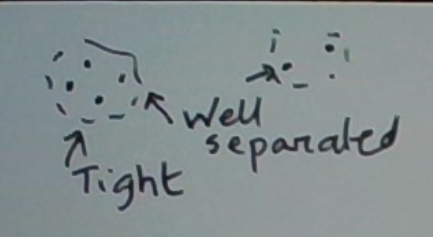
The clustering problem is to group a set of data points into clusters. Clusters should be internally tight. Clusters should also be well-separated.

Here is an example. Consider a geospatial map in which each pixel is green or yellow. A green pixel denotes a tree at that location. A yellow pixel denotes its absence. We’d like to cluster the trees into forests.
This is a representative example of a large class of clustering problems on geospatial data, at varying scales. For example, if we replace “green denoting a tree” with “red denoting a lit location”, we might hope to discover clusters of well-lit areas such as towns or neighborhoods.
In this post, we will cover the K-means clustering algorithm and its variants.
The K-means clustering algorithm requires fixing K, the number of clusters, in advance. This may seem like a serious limitation. In our example, how would we know the number of forests in advance?
That said, we can imagine some user interface that lets the user try out different values of K and see what forests get found? This interactive process might yet be useful.
The Algorithm
The K-means clustering algorithm works as follows. We are given the data set to be clustered, and a value of K. In our example, the data set would be the locations of the green pixels.
The algorithm initializes the K clusters (somehow). It then iteratively adjusts the clusters so long as they keep improving. We can stop the algorithm at any time. Or when the clusters stop changing (sufficiently).
How do we measure “clusters improving”? Let’s begin by noting that in K-means clustering clusters are represented by their means. (This explains the word “means” in the algorithm’s name.) In our trees example, a cluster’s mean is the associate forest’s center.
Next, we need the notion of how tight a cluster is. We will define a cluster’s width as the average distance of the cluster’s members from its mean. In our trees example, this is the average distance of a tree in a forest from the forest’s center. A rough proxy for the forest’s area.
A global measure of the tightness of the full set of clusters may then be defined as the sum of the widths of the clusters.
Next, let’s look at what happens inside an iteration. The algorithm tries to improve the current clustering. In two steps. First, it reassigns each data point to the cluster whose mean is closest to it. Next, it recomputes the cluster means from the updated assignments.
The intuition that an iteration (in which an assignment changes) improves the clustering is as follows. (This is not proof — just intuition!) In the first step, at least one data point got reassigned to a cluster whose center it is nearer to. This tends to reduce the width of one or both affected clusters. The second step, which recomputes the cluster means, often reduces the width further.
Example
Let’s illustrate this in the example below in which both effects come into play. We have 3 1D points to be clustered: 1, 5, and 6. Say the current clusters are {1, 5} and {6}. Their means are 3 and 6 respectively. In the next iteration 5 moves to the second cluster. This results in the clustering {1} and {5, 6} having means 1 and 5.5 respectively.
This shift is depicted below.
{1, 5}, {6} → {1}, {5, 6}
Let’s see how the cluster widths changed. The original clusters {1, 5} and {6} were 2 and 0 units wide respectively. The new clusters {1} and {5, 6} are 0 and 0.5 units wide respectively. So the summed widths reduced. That is, the overall clustering got tighter.
Finally, for completeness, let’s note that after the clusters have been initialized (before the iterations begin) their means need to be computed. This extra step is needed since step 1 of an iteration uses the means.
K-medians Clustering
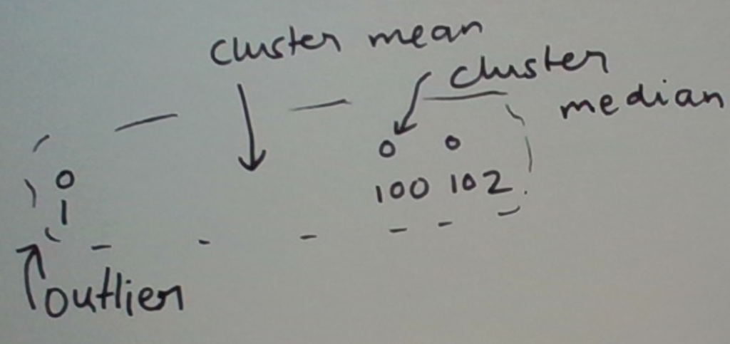
Consider the 1D data 1, 100, 102, 200 and say K = 2. What should be the two clusters? Either {{1, 100, 102}, {200}} or {{1}, {100,102, 200}}. In the first case 1 is an outlier; in the second case 200. The mean of a cluster with an outlier is skewed towards the outlier.
In the presence of outliers, a sensible variant of K-means clustering involves just replacing ‘mean’ with ‘median’. Nothing else changes.
Consider {1, 100, 102}. The mean is 67.66 whereas the median is 100. This is graphically depicted below.

Soft K-means Clustering: The EM algorithm
K-means clustering is a special case of a powerful statistical algorithm called EM. We will describe EM in the context of K-means clustering, calling it EMC. For contrast, we will denote k-means clustering as KMC.
EMC models a cluster as a probability distribution over the data space. Think of this as specifying a cluster by a soft membership function.
Take our trees example. Imagine that we are okay with elliptical forests (of which circular ones are special cases). We might model such a cluster as a two-dimensional Gaussian whose mean models the cluster’s center. Its covariance matrix captures the parameters that describe the shape of the ellipse (the major and minor axes and the tilt).
Before going further, let’s note that when we say elliptical clusters, this is just an approximation for visual insights. A cluster doesn’t have a hard boundary. Much like a mountain doesn’t have a hard boundary separating it from the plains. Nonetheless, as with a mountain, the imagined boundary is useful.
As in K-means clustering, the number of clusters is fixed in advance.
The next key concept is the probability model that describes the process of generating clusters. We call such a model a generative one.
The EMC generative model is a mixture whose components are the K individual cluster models. This mixture is parametrized by a distribution of mixing probabilities over the K clusters.
The generation process works as follows. We repeat the following independently as long as we like.
- Randomly sample a cluster, call it c, from C.
- Randomly sample a data point, call it x, from c’s distribution.
This results in a set of data points labeled with their cluster ids.
During the clustering process, the cluster ids of the data points are of course not known. The job of EMC is to find them.
In more detail, and a bit more generally, EMC’s aim is to learn the parameters of the various cluster models, together with the mixing probabilities, from the data. (We say “more generally” because this way we can also cluster new data that the algorithm hasn’t seen yet.)
The EMC algorithm’s steps
Just like K-means clustering, EMC works iteratively to improve the clustering. In fact, each iteration has the same two steps.
The two steps in an EMC iteration are more advanced versions of the corresponding steps in KMC. We’ll start by reviewing the KMC versions, then morph them into EMC ones. During the process, new ideas will emerge.
The first KMP step was to reassign the data points to the nearest clusters. The two words to focus on here are ‘reassign’ and ‘nearest’. Let’s look at ‘reassign’ first. As it turns out, first we have to abstract out a bit, to the word ‘assign’.
Cluster Assignments
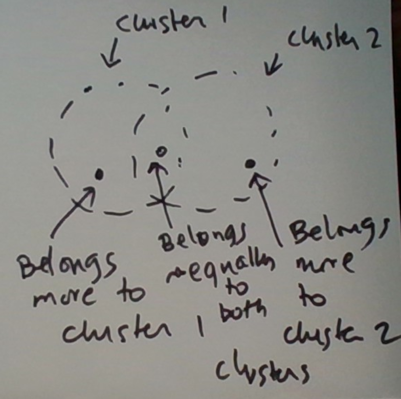
In KMC, the cluster assigned to a data point at any given time is unique. In EMC, a data point’s membership is modeled as a probability distribution over the various clusters. Thus the datum potentially belongs to multiple clusters, to a varying degree. This is graphically depicted below.

The KMC version is a special case in which the distribution’s mass is concentrated on one cluster.
How do we compute this probability distribution at any point in time? Actually, we could do it even for the KMC. Whereas the EMC’s version will be more accurate, let’s start by describing one from the KMC as it is simpler and we are on familiar ground.
Consider a datum x. We can compute the distance of x to every cluster. Next, we turn distances into membership scores which we call cluster affinities. One way to do this is to define data point x’s affinity for a cluster c at distance d from x to be 1/(d+p). Here p is a tiny positive number to avoid divide-by-zero. Next, we sum up these affinities. Finally, we divide each affinity by this sum. This gives us the soft cluster memberships of x as a probability distribution.
What we described above is fine for illustrative purposes but probably not effective enough for actual use. Simply put, cluster affinities can get overly diluted. That is, a single data point may belong to way too many clusters. Such diffusion can get in the way of trying to find a good clustering.
This issue can be mitigated by using softmax instead. This involves surgery on only the step in going from distance to affinity. Specifically, the affinity of distance d is defined as e^-d. Thus affinity drops exponentially with distance. Now we normalize as before.
Using the softmax this way produces a k-means like behavior. Simply put softmax is a better approximation to max than the function that came before it.
Bayesian Cluster Assignments
Whereas the softmax approach described above can be effective in practice, a more elaborate approach is below. Let c denote a cluster and x a data point. By Bayes rule,
P(c|x) = P(x|c)*P(c)/sum_c’ P(x|c’)*P(c’)
At any given point in time, we have an estimate of P(c). At any given point in time, we can also estimate P(x|c) as cluster c’s current probability model is fully specified. If, as in our trees example, a cluster’s model was a two-dimensional Gaussian, fully specified just means that the cluster’s mean and covariance matrices have specific values.
Completing The First Step’s Description
So we have all the information to compute P(c|x). Note that this approach takes into account the cluster sizes as well. (Think of P(c) as proportional to c’s size.) So if two clusters were equally near a data point, the data point would favor the larger cluster.
The Second Step
The second step in KMC was to recompute the cluster means. In EMC, this generalizes to “reestimate the model parameters”. These include the parameters of the various cluster models as well as the mixing probabilities of the mixture model.
We’ll illustrate this step for the case in which the cluster models are two-dimensional Gaussians. This will immediately apply to our trees example.
Let’s start with reestimating a cluster’s mean. In KMC, this was just the mean of the data points in the cluster. In EMC, a data point can be in multiple clusters to a varying degree so this needs some generalization.
Fortunately, the generalization is intuitively easy to describe. In EMC a data point x contributes to the mean of cluster c with weight proportional to P(c|x). In more detail,
mean(c) = sum_x P(c|x)*x/ sum_x P(c|x)
Let’s illustrate this in the KMC special case. P(c|x) is 1 for c’s members and 0 for the rest. So mean(c) = sum_{x in c} x/sum_{x in c} 1 = sum_{x in c} x/cluster size(c) which is exactly what we had.
In summary, in KMC a data point contributes to the mean of its unique cluster. In EMC a data point contributes to the means of potentially multiple clusters, with strengths based on the involved cluster affinities.
The covariance matrix of a cluster may be estimated similarly, albeit the details are more involved.
The mixing probabilities are reestimated as follows.
P(c) = sum_x P(c|x)/sum_{x, c’} P(c’|x)
Think of P(c) as the sum of the weighted votes it receives divided by the sum of the weighted votes all clusters receive.
Example: A Mixture Of Two Gaussians
EMC is a complex algorithm. An example will help.
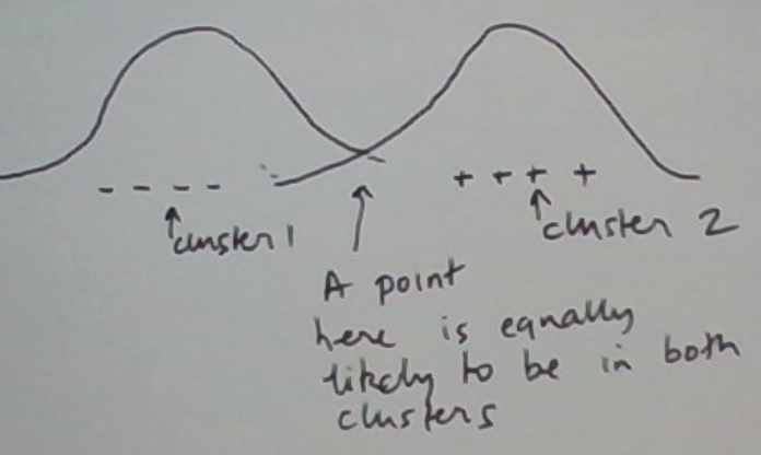
We will operate on a single dimension and set K = 2.We will model each cluster as a Gaussian.
The situation is graphically depicted below.

For numerical calculations let’s restrict the situation further. Let’s consider the same 3 data points 1, 5, and 6 and the same initial clusters {1, 5} and {6}. In EMC, we also need to initialize the model parameters. Let’s just estimate them from the initial clusters.
Let’s set the cluster posterior probabilities from the initial clustering. That is, as, in KMC, a datum determines its cluster uniquely. Next, we compute the cluster means to be 3 and 6 respectively. The cluster standard deviations are 2 and 0 respectively.
The second cluster’s standard deviation of 0 poses a slight problem. The resulting Gaussian is degenerate. We can’t use it.
We’ll patch this situation as follows. We will add n copies of 1, 5, and 6, where n >> 1. To these, we will add a few points sampled randomly from a Gaussian whose mean and standard deviation are the corresponding statistics of the sample 1, 5, and 6.
Now we will initialize the clusters from this expanded data. The reason for n >> 1 is because we want 1, 5, and 6 to remain the dominant numbers.
This may be interpreted as a Bayesian approach in which we have incorporated a prior that the standard deviations of all clusters must be positive. While we are at it, let’s tack on another sensible prior: that neither cluster is empty, i.e. its mixing probability is 0.
For illustration purposes let’s wish away the synthetic data we added. We will bring it in whenever it is relevant. That is, let’s start as before, with three points 1, 5, and 6, and the initial clustering {1, 5} and {6}.
We get the cluster means to be approximately 3 and 6 respectively. (This is because the synthetic data has some effect.) The cluster standard deviations are approximately 2 and positive respectively.
Next, we update the posterior probabilities of the two clusters. For visual convenience, we’ll use the distance versions of the update formulae.
The before and after depictions below will help illustrate the update process. First, let’s depict the data points.
x 1 5 6
Next, let’s see the probabilities of cluster 1 before the update. (P(2|x) is 1-P(1|x).)
x      1            5 6
P(1|x) 1            1 0
Next, let’s see the updated probabilities of cluster 1 based on their distances.
x      1            5 6
P(1|x) ~1          ~0 0
The bold-faced one changed the most. Effectively we softly moved data point 5 from cluster 1 to cluster 2.
Now each data point’s cluster probabilities are concentrated on one cluster. Plus nearby points (5 and 6) have high posteriors for the same cluster. So the clustering is in a happy state.
Summary
In this post, we described a well-known and classical algorithm for clustering known as K-means clustering. We also covered an advanced variant called soft k-means clustering and a robust variant that uses median instead of mean.


