TL;DR: Graph neural networks exploit relational inductive biases for data that come in the form of a graph. However, in many cases we do not have the graph readily available. Can graph deep learning still be applied in this case? In this post, I draw parallels between recent works on latent graph learning and older techniques of manifold learning.
The past few years have witnessed a surge of interest in developing ML methods for graph-structured data. Such data naturally arises in many applications such as social sciences (e.g. the Follow graph of users on Twitter or Facebook), chemistry (where molecules can be modelled as graphs of atoms connected by bonds), or biology (where interactions between different biomolecules are often modelled as a graph referred to as the interactome). Graph neural networks (GNNs), which I have covered extensively in my previous posts, are a particularly popular method of learning on such graphs by means of local operations with shared parameters exchanging information between adjacent nodes.
In some settings, however, we do not have the luxury of being given a graph to work with as input. This is a typical situation for many biological problems, where graphs such as protein-to-protein interaction are only partially known in the best case, as the experiments by which interactions are discovered are expensive and noisy. We are therefore interested in inferring the graph from the data and applying a GNN on it [1] — I call this setting “latent graph learning” [2]. The latent graph might be application-specific and optimised for the downstream task. Furthermore, sometimes such a graph might be even more important than the task itself, as it may convey important insights about the data and offer a way to interpret the results.
Away of thinking of latent graph learning is that of a graph with an empty edge set. In this setting, the input is provided as a point cloud in some high-dimensional feature space. Unlike methods for deep learning on sets such as PointNet [3], which apply some shared learnable point-wise function to each point, we also seek to pass information across points. This is done by message passing on a graph constructed from the point features themselves.
The first architecture of this kind, Dynamic Graph CNN (DGCNN) [4], was developed by Yue Wang from MIT, with whom I had the pleasure to collaborate during my sabbatical at that institution. Motivated by problems in computer graphics dealing with the analysis of 3D point clouds, the idea was to use the graph as a coarse representation of the local smooth manifold structure underlying a point cloud. A key observation of Yue was that the graph does not need to stay the same throughout the neural network, and in fact it can and should be updated dynamically — hence the name of the method. The following figure from our paper illustrates why this might be useful in computer graphics problems:
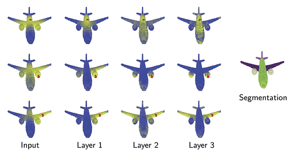
One of the limitations of DGCNNs was that the same space is used to construct the graph and the features on that graph. In a recent work with Anees Kazi from TUM and my postdoc Luca Cosmo, we proposed a new architecture called Differentiable Graph Module (DGM) [5] extending DGCNN by decoupling the graph and feature construction, as shown in the following figure:

DGM showed impressive results when applied to problems from the medical domain, such as disease prediction from brain imaging data. In these tasks, we are provided with the electronic health records of multiple patients, including demographic features (such as age, sex, etc) and brain imaging features, and attempt to predict whether a patient suffers from a neurological disease. Previous works showed the application of GNNs to such tasks using diffusion on a “patient graph” constructed by hand from the demographic features [6]. DGM offers the advantage of learning the graph, which possibly conveys insight into how certain features depend on each other for the specific diagnosis task. As a bonus, DGM also beat DGCNN in its game of point cloud classification, albeit only slightly.
DGCNN and DGM bear conceptual similarity to a family of algorithms called manifold learning or non-linear dimensionality reduction, which were extremely popular in machine learning when I was a student in the 2000s, and are still used for data visualisation. The assumption underlying manifold learning methods is that of the data having an intrinsic low-dimensional structure. Though the data can be represented in a space of hundreds or even thousands of dimensions, it only has a few degrees of freedom, as shown in the following example:
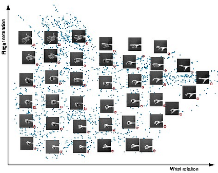
The purpose of manifold learning is to capture these degrees of freedom (by reconstructing the underlying “manifold”, hence the name [7]) and reduce the dimensionality of the data to its intrinsic dimension. The important difference from linear dimensionality reduction such as PCA is that, due to the non-Euclidean structure of the data, there might be no possibility to recover the manifold by means of a linear projection [8]:
One of the challenges is that the construction of the graph is decoupled from the ML algorithm, and sometimes delicate parameter tuning (e.g. the number of neighbours or the neighbourhood radius) is needed in order to figure out how to build the graph to make the downstream task work well. Perhaps a far more serious drawback of manifold learning algorithms is that data rarely presents itself as low-dimensional in its native form. When dealing with images, for example, various handcrafted feature extraction techniques had to be used as pre-processing steps.
Graph deep learning offers a modern take on this process, by replacing this three-stage process outlined above with a single graph neural network. In dynamic graph CNNs or DGM, for instance, the construction of the graph and the learning are part of the same architecture:
The appeal of this approach is the possibility to combine the treatment of individual data points and the space in which they reside in the same pipeline. In the example of images, one could use traditional CNNs to extract the visual features from each image and use a GNN to model the relations between them. This approach was used in the work of my PhD student Jan Svoboda: he proposed a graph-based regularisation layer (called PeerNet) for CNNs that allows to exchange information between multiple images [12]. PeerNets bear similarity to non-local means filters [13] in the way they aggregate information from multiple locations, with the main difference that the aggregation happens across multiple images rather than a single one. We showed that such a regularisation dramatically reduces the effect of adversarial perturbations to which standard CNNs are highly susceptible [14].
There are many other interesting applications of latent graph learning. One is few-shot learning, where graph-based techniques can help generalise from a few examples. Few-shot learning is becoming increasingly important in computer vision where the cost of data labelling is significant [5]. Another field is biology, where one often observes experimentally expression levels of biomolecules such as proteins and tries to reconstruct their interaction and signalling networks [15]. Third problem is the analysis of physical systems where a graph can describe interactions between multiple objects [16]. In particular, high-energy physicists dealing with complex particle interactions have recently been showing keen interest in graph-based approaches [17]. Last but not least are problems in NLP, where graph neural networks can be seen as generalisations of the transformer architecture. Many of the mentioned problems also raise questions on incorporating priors on the graph structure, which is still largely open: for example, one may wish to force the graph to obey certain construction rules or be compatible with some statistical model [18].
I believe that latent graph learning, while not entirely new, offers a new perspective on old problems. It is for sure an interesting setting of graph ML problems, providing a new playground for GNN researchers.
[1] A slightly different but related class of methods seeks to decouple the graph provided as input from the computational graph used for message passing in graph neural networks, see e.g. J. Halcrow et al. Grale: Designing networks for graph learning (2020). arXiv:2007.12002. There are multiple reasons why one may wish to do it, one of which is breaking the bottlenecks related to the exponential growth of the neighbourhood size in some graphs, as shown by U. Alon and E. Yahav, On the bottleneck of graph neural networks and its practical implications (2020). arXiv:2006.05205.
[2] Problems of reconstructing graphs underlying some data were considered in the signal processing context in the PhD thesis of Xiaowen Dong, in whose defence committee I took part in May 2014, just a few days before the birth of my son. X. Dong et al. Learning graphs from data: A signal representation perspective (2019), IEEE Signal Processing Magazine 36(3):44–63 presents a good summary of this line of work. A more recent incarnation of these approaches from the perspective of network games is the work of Y. Leng et al. Learning quadratic games on networks (2020). Proc. ICML, on whose PhD committee at MIT I was earlier this year.
[3] C. Qi et al. PointNet: Deep learning on point sets for 3D classification and segmentation (2017), Proc. CVPR. PointNet is an architecture for deep learning on sets, where a shared function is applied to the representation of each point, and can be considered as a trivial case of a GNN applied to a graph with empty edge set.
[4] Y. Wang et al. Dynamic graph CNN for learning on point clouds (2019). ACM Trans. Graphics 38(5):146. This paper has become quite popular in the computer graphics community and is often used as a baseline for point cloud methods. Ironically, it was rejected from SIGGRAPH in 2018 and was presented at the same conference only two years later after having gathered over 600 citations.
[5] A. Kazi et al., Differentiable Graph Module (DGM) for graph convolutional networks (2020) arXiv:2002.04999. We show multiple applications, including medical imaging, 3D point cloud analysis, and few shot learning. See also our paper L. Cosmo et al. Latent patient network learning for automatic diagnosis (2020). Proc. MICCAI, focusing on a medical application of this method. Anees was a visiting PhD student in my group at Imperial College in 2019.
[6] To the best of my knowledge, the first use of GNNs for brain disease prediction is by S. Parisot et al. Disease prediction using graph convolutional networks: application to autism spectrum disorder and Alzheimer’s disease (2017). Proc. MICCAI. The key drawback of this approach was a handcrafted construction of the graph from demographic features.
[7] Formally speaking, it is not a “manifold” in the differential geometric sense of the term, since for example the local dimension can vary at different points. However, it is a convenient metaphor.
[8] The more correct term is “non-Euclidean” rather than “non-linear”.
[9] J. B. Tenenbaum et al., A global geometric framework for nonlinear dimensionality reduction (2000), Science 290:2319–2323. Introduced the Isomap algorithm that embeds the data manifold by trying to preserve the geodesic distances on it, approximated using a k-NN graph. Geodesic distances on the graph are the lengths of the shortest paths connecting any pair of points, computed by means of the Dijkstra algorithm. Endowed with such a distance metric, the dataset is considered as a (non-Euclidean) metric space. A configuration of points in a low-dimensional space whose pairwise Euclidean distances are equal to the graph geodesic distances is known as isometric embedding in metric geometry. Usually, isometric embeddings do not exist and one has to resort to an approximation that preserves the distances the most in some sense. One way of computing such an approximation is by means of multidimensional scaling (MDS) algorithms.
[10] S. T. Roweis and L. K. Saul, Nonlinear dimensionality reduction by locally linear embedding (2000). Science 290:2323–2326.
[11] M, Belkin and P. Niyogi, Laplacian eigenmaps and spectral techniques for embedding and clustering (2001). Proc. NIPS.
[12] J. Svoboda et al. PeerNets: Exploiting peer wisdom against adversarial attacks (2019), Proc. ICLR uses GNN module that aggregates information from multiple images to reduce the sensitivity of CNNs to adversarial perturbations of the input.
[13] Non-local means is a non-linear image filtering technique introduced by A. Buades et al., A non-local algorithm for image denoising (2005), Proc. CVPR. It can be seen as a precursor to modern attention mechanisms used in deep learning. Non-local means itself is a variant of edge-preserving diffusion methods such as the Beltrami flow proposed by my PhD advisor Ron Kimmel in the paper R. Kimmel et al., From high energy physics to low level vision (1997), Proc. Scale-Space Theories in Computer Vision, or the bilateral filter from C. Tomasi and R. Manduchi, Bilateral filtering for gray and color images (1998). Proc. ICCV.
[14] Adversarial perturbation is a carefully constructed input noise that significantly reduces the performance of CNNs e.g. in image classification. This phenomenon was described in C. Szegedy et al. Intriguing properties of neural networks (2014), Proc. ICLR, and resulted in multiple follow-up works that showed bizarre adversarial attacks as extreme as changing a single pixel (J. Su et al. One pixel attack for fooling deep neural networks (2017), arXiv:1710.08864) or data-independent “universal” perturbations (S. M. Moosavi-Dezfooli et al., Universal adversarial perturbations (2017), Proc. CVPR).
[15] Y. Yu et al., DAG-GNN: DAG structure learning with graph neural networks (2019). Proc. ICML.
[16] T. Kipf et al., Neural relational inference for interaction systems (2019). Proc. ICML. Recovers a graph “explaining” the physics of a system by using a variational autoencoder, in which the latent vectors represent the underlying interaction graph and the decoder is a graph neural network.
[17] The use of GNNs in high-energy physics is a fascinating topic worth a separate post. Together with my PhD student Federico Monti we have worked with the IceCube collaboration developing probably the first GNN-based approach for particle physics. Our paper N. Choma, F. Monti et al., Graph neural networks for IceCube signal classification (2018), Proc. ICMLA, where we used the MoNet architecture for astrophysical neutrino classification, got the best paper award. In a more recent work, S. R. Qasim et al., Learning representations of irregular particle-detector geometry with distance-weighted graph networks (2019), European Physical Journal C 79, used a variant of DGCNN similar to DGM called GravNet for particle reconstruction.
[18] A somewhat related class of approaches are generative graph models, see e.g. Y. Li et al, Learning deep generative models of graphs (2018). arXiv:1803.03324. One of the applications is generating molecular graphs of chemical compounds that adhere to strict construction rules.
[19] There are many more works on latent graph learning papers that have appeared in the past couple of years — if I omit some, this is because my goal is not to be exhaustive but rather to show a principle. I will refer to one additional work of L. Franceschi et al. Learning discrete structures for graph neural networks (2019). Proc. ICML, which also mentions the relation to Isomap and manifold learning techniques.
I am grateful to Ben Chamberlain, Xiaowen Dong, Fabrizio Frasca, Anees Kazi, and Yue Wang for proof-reading this post, and to Gal Mishne for pointing to the origins of the Swiss roll. See my other posts on Medium, or follow me on Twitter.


