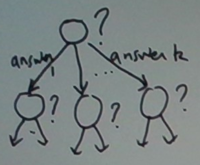
In the context of supervised learning, a decision tree is a tree for predicting the output for a given input. We start from the root of the tree and ask a particular question about the input. Depending on the answer, we go down to one or another of its children. The child we visit is the root of another tree. So we repeat the process, i.e. ask another question here. Eventually, we reach a leaf, i.e. a node with no children. This node contains the final answer which we output and stop.
This process is depicted below.
Let’s see an example.
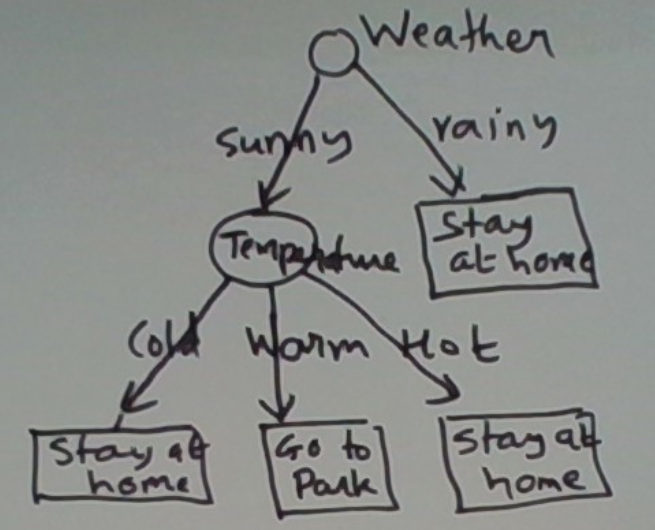
In machine learning, decision trees are of interest because they can be learned automatically from labeled data. A labeled data set is a set of pairs (x, y). Here x is the input vector and y the target output.
Below is a labeled data set for our example.
Weather Temperature Action
Sunny   Warm        Go to park
Sunny   Cold        Stay at home
Sunny   Hot         Stay at home
Rainy   Warm        Stay at home
Rainy   Cold        Stay at home
Why Decision Trees
Learned decision trees often produce good predictors. Because they operate in a tree structure, they can capture interactions among the predictor variables. (This will register as we see more examples.)
The added benefit is that the learned models are transparent. That is, we can inspect them and deduce how they predict. By contrast, neural networks are opaque. Deep ones even more so.
Of course, when prediction accuracy is paramount, opaqueness can be tolerated. Decision trees cover this too. Ensembles of decision trees (specifically Random Forest) have state-of-the-art accuracy.
So either way, it’s good to learn about decision tree learning.
Learning Decision Trees
Okay, let’s get to it. We’ll focus on binary classification as this suffices to bring out the key ideas in learning. For completeness, we will also discuss how to morph a binary classifier to a multi-class classifier or to a regressor.
The pedagogical approach we take below mirrors the process of induction. We’ll start with learning base cases, then build out to more elaborate ones.
Learning Base Case 1: Single Numeric Predictor
Consider the following problem. The input is a temperature. The output is a subjective assessment by an individual or a collective of whether the temperature is HOT or NOT.
Let’s depict our labeled data as follows, with – denoting NOT and + denoting HOT. The temperatures are implicit in the order in the horizontal line.
- - - - - + + + + +
This data is linearly separable. All the -s come before the +s.
In general, it need not be, as depicted below.
- - - - - + - + - - - + - + + - + + - + + + + + + + +
Perhaps the labels are aggregated from the opinions of multiple people. There might be some disagreement, especially near the boundary separating most of the -s from most of the +s.
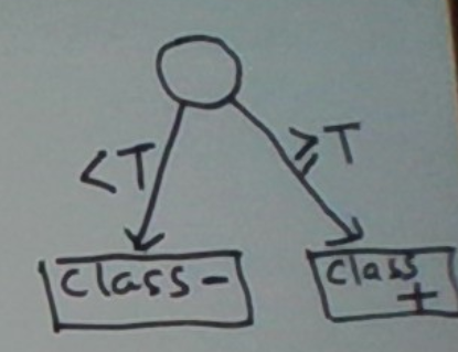
Our job is to learn a threshold that yields the best decision rule. What do we mean by “decision rule”. For any threshold T, we define this as
IF temperature < T
  return NOT
ELSE
  return HOT
The accuracy of this decision rule on the training set depends on T.
The objective of learning is to find the T that gives us the most accurate decision rule. Such a T is called an optimal split.
In fact, we have just seen our first example of learning a decision tree. The decision tree is depicted below.
Learning Base Case 2: Single Categorical Predictor
Consider season as a predictor and sunny or rainy as the binary outcome. Say we have a training set of daily recordings. For each day, whether the day was sunny or rainy is recorded as the outcome to predict. The season the day was in is recorded as the predictor.
This problem is simpler than Learning Base Case 1. The predictor has only a few values. The four seasons. No optimal split to be learned. It’s as if all we need to do is to fill in the ‘predict’ portions of the case statement.
case season
when summer: Predict sunny
when winter: Predict rainy
when fall: ??
when spring: ??
That said, we do have the issue of “noisy labels”. This just means that the outcome cannot be determined with certainty. Summer can have rainy days.
This issue is easy to take care of. At a leaf of the tree, we store the distribution over the counts of the two outcomes we observed in the training set. This is depicted below.
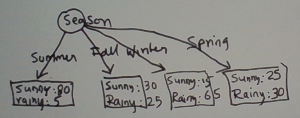
Say the season was summer. The relevant leaf shows 80: sunny and 5: rainy. So we would predict sunny with a confidence 80/85.
Learning General Case 1: Multiple Numeric Predictors
Not surprisingly, this is more involved.
We start by imposing the simplifying constraint that the decision rule at any node of the tree tests only for a single dimension of the input.
Call our predictor variables X1, …, Xn. This means that at the tree’s root we can test for exactly one of these. The question is, which one?
We answer this as follows. For each of the n predictor variables, we consider the problem of predicting the outcome solely from that predictor variable. This gives us n one-dimensional predictor problems to solve. We compute the optimal splits T1, …, Tn for these, in the manner described in the first base case. While doing so we also record the accuracies on the training set that each of these splits delivers.
At the root of the tree, we test for that Xi whose optimal split Ti yields the most accurate (one-dimensional) predictor. This is depicted below.
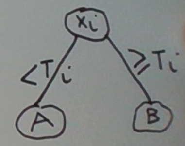
So now we need to repeat this process for the two children A and B of this root. Towards this, first, we derive training sets for A and B as follows. The training set for A (B) is the restriction of the parent’s training set to those instances in which Xi is less than T (>= T). Let’s also delete the Xi dimension from each of the training sets.
Now we have two instances of exactly the same learning problem. So we recurse.
And so it goes until our training set has no predictors. Only binary outcomes. The node to which such a training set is attached is a leaf. Nothing to test. The data on the leaf are the proportions of the two outcomes in the training set. This suffices to predict both the best outcome at the leaf and the confidence in it.
Learning General Case 2: Multiple Categorical Predictors
Here we have n categorical predictor variables X1, …, Xn. As we did for multiple numeric predictors, we derive n univariate prediction problems from this, solve each of them, and compute their accuracies to determine the most accurate univariate classifier. The predictor variable of this classifier is the one we place at the decision tree’s root.
Next, we set up the training sets for this root’s children.
There is one child for each value v of the root’s predictor variable Xi. The training set at this child is the restriction of the root’s training set to those instances in which Xi equals v. We also delete attribute Xi from this training set.
Now we recurse as we did with multiple numeric predictors.
Example
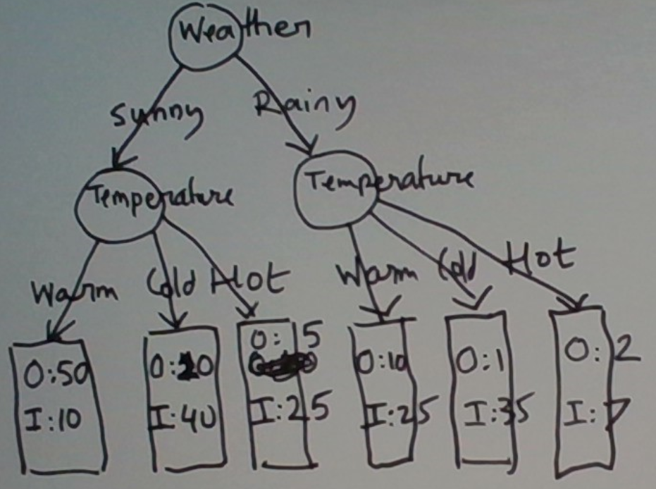
Let’s illustrate this learning on a slightly enhanced version of our first example, below. We’ve named the two outcomes O and I, to denote outdoors and indoors respectively. We’ve also attached counts to these two outcomes. A row with a count of o for O and i for I denotes o instances labeled O and i instances labeled I.
Weather Temperature Action
Sunny   Warm        O (50), I (10)
Sunny   Cold        O (10), I (40)
Sunny   Hot         O (5), I (30)
Rainy   Warm        O (10), I (25)
Rainy   Cold        O (1), I (35)
Rainy   Hot         O (2), I(7)
So what predictor variable should we test at the tree’s root? Well, weather being rainy predicts I. (That is, we stay indoors.) Weather being sunny is not predictive on its own. Now consider Temperature. Not surprisingly, the temperature is hot or cold also predicts I.
Which variable is the winner? Not clear. Let’s give the nod to Temperature since two of its three values predict the outcome. (This is a subjective preference. Don’t take it too literally.)
Now we recurse.
The final tree that results is below.
Mixed Predictor Variables
What if we have both numeric and categorical predictor variables? A reasonable approach is to ignore the difference. To figure out which variable to test for at a node, just determine, as before, which of the available predictor variables predicts the outcome the best. For a numeric predictor, this will involve finding an optimal split first.
The Learning Algorithm: Abstracting Out The Key Operations
Let’s abstract out the key operations in our learning algorithm. These abstractions will help us in describing its extension to the multi-class case and to the regression case.
The key operations are
- Evaluate how accurately any one variable predicts the response.
- Derive child training sets from those of the parent.
Multi-class Case
What if our response variable has more than two outcomes? As an example, say on the problem of deciding what to do based on the weather and the temperature we add one more option: go to the Mall.
Fundamentally nothing changes. Adding more outcomes to the response variable does not affect our ability to do operation 1. (The evaluation metric might differ though.) Operation 2 is not affected either, as it doesn’t even look at the response.
Regression
What if our response variable is numeric? Here is one example. Predict the day’s high temperature from the month of the year and the latitude.
Can we still evaluate the accuracy with which any single predictor variable predicts the response? This raises a question. How do we even predict a numeric response if any of the predictor variables are categorical?
Let’s start by discussing this. First, we look at
Base Case 1: Single Categorical Predictor Variable
For each value of this predictor, we can record the values of the response variable we see in the training set. A sensible prediction is the mean of these responses.
Let’s write this out formally. Let X denote our categorical predictor and y the numeric response. Our prediction of y when X equals v is an estimate of the value we expect in this situation, i.e. E[y|X=v].
Let’s see a numeric example. Consider the training set
X A A B B
y 1 2 4 5
Our predicted ys for X = A and X = B are 1.5 and 4.5 respectively.
Base Case 2: Single Numeric Predictor Variable
For any particular split T, a numeric predictor operates as a boolean categorical variable. So the previous section covers this case as well.
Except that we need an extra loop to evaluate various candidate T’s and pick the one which works the best. Speaking of “works the best”, we haven’t covered this yet. We do this below.
Evaluation Metric
Both the response and its predictions are numeric. We just need a metric that quantifies how close to the target response the predicted one is. A sensible metric may be derived from the sum of squares of the discrepancies between the target response and the predicted response.
General Case
We have covered operation 1, i.e. evaluating the quality of a predictor variable towards a numeric response. Operation 2, deriving child training sets from a parent’s, needs no change. As noted earlier, this derivation process does not use the response at all.
The Response Predicted At A Leaf
As in the classification case, the training set attached at a leaf has no predictor variables, only a collection of outcomes. As noted earlier, a sensible prediction at the leaf would be the mean of these outcomes. So this is what we should do when we arrive at a leaf.
Modeling Tradeoffs
Consider our regression example: predict the day’s high temperature from the month of the year and the latitude.
Consider the month of the year. We could treat it as a categorical predictor with values January, February, March, … Or as a numeric predictor with values 1, 2, 3, …
What are the tradeoffs? Treating it as a numeric predictor lets us leverage the order in the months. February is near January and far away from August. That said, how do we capture that December and January are neighboring months? 12 and 1 as numbers are far apart.
Perhaps more importantly, decision tree learning with a numeric predictor operates only via splits. That would mean that a node on a tree that tests for this variable can only make binary decisions. By contrast, using the categorical predictor gives us 12 children. In principle, this is capable of making finer-grained decisions.
Now consider latitude. We can treat it as a numeric predictor. Or as a categorical one induced by a certain binning, e.g. in units of + or – 10 degrees. The latter enables finer-grained decisions in a decision tree.
Summary
In this post, we have described learning decision trees with intuition, examples, and pictures. We have covered both decision trees for both classification and regression problems. We have also covered both numeric and categorical predictor variables.
Further Reading


