Machine Learning Algorithms In Layman’s Terms

This series of posts is me sharing with the world how I would explain all the machine learning topics I come across on a regular basis…to my grandma. Some get a bit in-depth, others less so, but all I believe are useful to a non-Data Scientist.

The topics in this first part are:

In the upcoming parts of this series, I’ll be going over:

Decision Trees
Random Forest
SVM
Naive Bayes
RNNs & CNNs
K-NN
K-Means
DBScan
Hierarchical Clustering
Agglomerative Clustering
eXtreme Gradient Boosting
AdaBoost

Before we start, a quick aside on the difference(s) between algorithms and models, taken from this great Quora post:

“a model is like a Vending Machine, which given an input (money), will give you some output (a soda can maybe) . . . An algorithm is what is used to train a model, all the decisions a model is supposed to take based on the given input, to give an expected output. For example, an algorithm will decide based on the dollar value of the money given, and the product you chose, whether the money is enough or not, how much balance you are supposed to get [back], and so on.”

To summarize, an algorithm is the mathematical life force behind a model. What differentiates models are the algorithms they employ, but without a model, an algorithm is just a mathematical equation hanging out with nothing to do.

With that, onwards!

Gradient Descent / Line of Best Fit

(While this first one isn’t traditionally thought of as a machine-learning algorithm, understanding gradient descent is vital to understanding how many machine learning algorithms work and are optimized.)

Me-to-grandma:

“Basically, gradient descent helps us get the most accurate predictions based on some data.

Let me explain a bit more – let’s say you have a big list of the height and weight of every person you know. And let’s say you graph that data. It would probably look something like this:

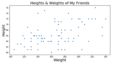
Our fake height and weight data set (…strangely geometric)

Now let’s say there’s a local guessing competition where the person to guess someone’s weight correctly, given their height, gets a cash prize. Besides using your eyes to size the person up, you’d have to rely pretty heavily on the list of heights and weights you have at your disposal, right?

So, based on the graph of your data above, you could probably make some pretty good predictions if only you had a line on the graph that showed the trend of the data. With such a line, if you were given someone’s height, you could just find that height on the x-axis, go up until you hit your trend line, and then see what the corresponding weight is on the y-axis, right?

But how in the world do you find that perfect line? You could probably do it manually, but it would take forever. That’s where gradient descent comes in!

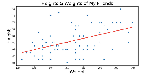
Our “line of best fit” is in red above.

It does this by trying to minimize something called RSS (the residual sum of squares), which is basically the sum of the squares of the differences between our dots and our line, i.e. how far away our real data (dots) is from our line (red line). We get a smaller and smaller RSS by changing where our line is on the graph, which makes intuitive sense — we want our line to be wherever it’s closest to the majority of our dots.

We can actually take this further and graph each different line’s parameters on something called a cost curve. Using gradient descent, we can get to the bottom of our cost curve. At the bottom of our cost curve is our lowest RSS!

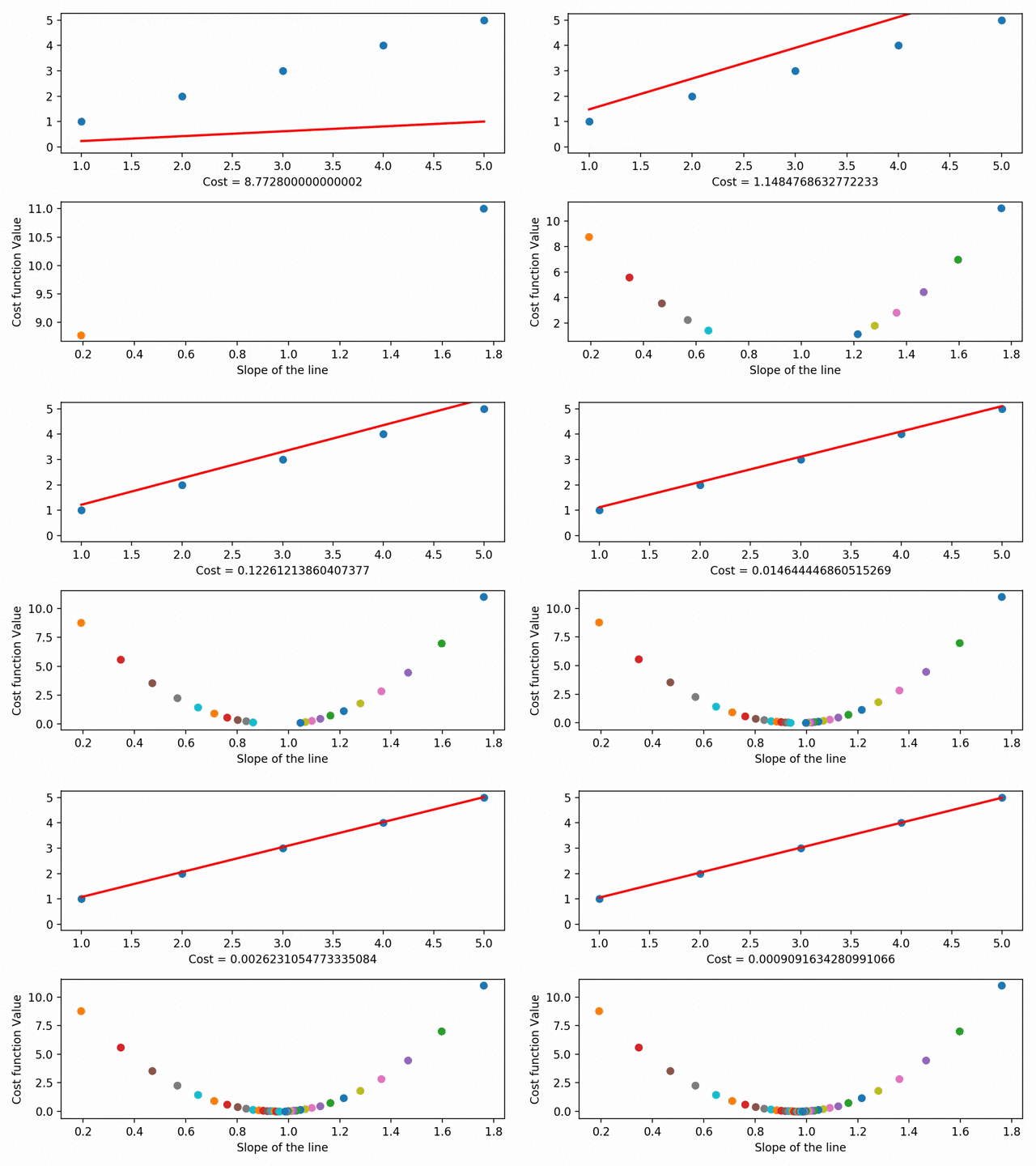
Gradient Descent visualized (using MatplotLib ), from the incredible Data Scientist Bhavesh Bhatt

There are more granular aspects of gradient descent like “step sizes” (i.e. how fast we want to approach the bottom of our skateboard ramp) and “learning rate” (i.e. what direction we want to take to reach the bottom), but in essence: gradient descent gets our line of best fit by minimizes the space between our dots and our line of best fit. Our line of best fit, in turn, allows us to make predictions!”

Linear Regression

Me-to-grandma:

“Super simply, linear regression is a way we analyze the strength of the relationship between 1 variable (our “outcome variable”) and 1 or more other variables (our “independent variables”).

A hallmark of linear regression, like the name implies, is that the relationship between the independent variables and our outcome variable is linear. For our purposes, all that means is that when we plot the independent variable(s) against the outcome variable, we can see the points start to take on a line-like shape, like they do below.

(If you can’t plot your data, a good way to think about linearity is by answering the question: does a certain amount of change in my independent variable(s) result in the same amount of change in my outcome variable? If yes, your data is linear!)

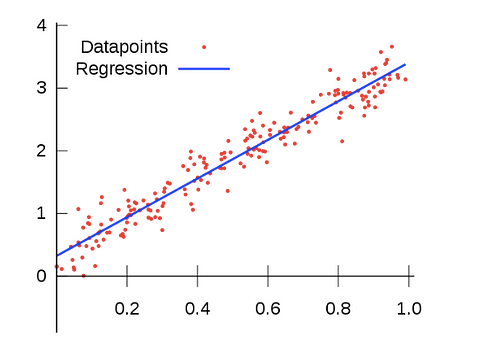
This looks a ton like what we did above! That’s because the line of best fit we discussed before IS our “regression line” in linear regression. The line of best fit shows us the best possible linear relationship between our points. That, in turn, allows us to make predictions.

Another important thing to know about linear regression is that the outcome variable, or the thing that changes depending on how we change our other variables, is always continuous. But what does that mean?

Let’s say we wanted to measure what effect elevation has on rainfall in New York State: our outcome variable (or the variable we care about seeing a change in) would be rainfall, and our independent variable would be elevation. With linear regression, that outcome variable would have to be specifically how many inches of rainfall, as opposed to just a True/False category indicating whether or not it rained at x elevation. That is because our outcome variable has to be continuous — meaning that it can be any number (including fractions) in a range of numbers.

The coolest thing about linear regression is that it can predict things using the line of best fit that we spoke about before! If we run a linear regression analysis on our rainfall vs. elevation scenario above, we can find the line of best fit like we did in the gradient descent section (this time shown in blue), and then we can use that line to make educated guesses as to how much rain one could reasonably expect at some elevation.”

Ridge & LASSO Regression

Me, continuing to hopefully-not-too-scared-grandma:

“So linear regression’s not that scary, right? It’s just a way to see what effect something has on something else. Cool.

Now that we know about simple linear regression, there are even cooler linear regression-like things we can discuss, like ridge regression.

Like gradient descent’s relationship to linear regression, there’s one back-story we need to cover to understand ridge regression, and that’s regularization.

Simply put, data scientists use regularization methods to make sure that their models only pay attention to independent variables that have a significant impact on their outcome variable.

You’re probably wondering why we care if our model uses independent variables that don’t have an impact. If they don’t have an impact, wouldn’t our regression just ignore them? The answer is no! We can get more into the details of machine learning later, but basically we create these models by feeding them a bunch of “training” data. Then, we see how good our models are by testing them on a bunch of “test” data. So, if we train our model with a bunch of independent variables, with some that matter and some that don’t, our model will perform super well on our training data (because we are tricking it to think all of what we fed it matters), but super poorly on our test data. This is because our model isn’t flexible enough to work well on new data that doesn’t have every. single. little. thing we fed it during the training phase. When this happens, we say that the model is “overfit.”

To understand over-fitting, let’s look at a (lengthy) example:

Let’s say you’re a new mother and your baby boy loves pasta. As the months go by, you make it a habit to feed your baby pasta with the kitchen window open because you like the breeze. Then your baby’s cousin gets him a onesie, and you start a tradition of only feeding him pasta when he’s in his special onesie. Then you adopt a dog who diligently sits beneath the baby’s highchair to catch the stray noodles while he’s eating his pasta . At this point, you only feed your baby pasta while he’s wearing the special onesie …and the kitchen window’s open …and the dog is underneath the highchair. As a new mom you naturally correlate your son’s love of pasta with all of these features: the open kitchen window, the onesie, and the dog. Right now, your mental model of the baby’s feeding habits is pretty complex!

One day, you take a trip to grandma’s. You have to feed your baby dinner (pasta, of course) because you’re staying the weekend. You go into a panic because there is no window in this kitchen, you forgot his onesie at home, and the dog is with the neighbors! You freak out so much that you forget all about feeding your baby his dinner and just put him to bed.

Wow. You performed pretty poorly when you were faced with a scenario you hadn’t faced before. At home you were perfect at it, though! It doesn’t make sense!

After revisiting your mental model of your baby’s eating habits and disregarding all the “noise,” or things you think probably don’t contribute to your boy actuallyloving pasta, you realize that the only thing that really matters is that it’s cooked by you.

The next night at grandma’s you feed him his beloved pasta in her windowless kitchen while he’s wearing just a diaper and there’s no dog to be seen. And everything goes fine! Your idea of why he loves pasta is a lot simpler now.

That is exactly what regularization can do for a machine learning model.

So, regularization helps your model only pay attention to what matters in your data and gets rid of the noise.

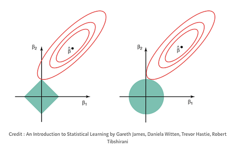
On the left: LASSO regression (you can see that the coefficients, represented by the red rungs, can equal zero when they cross the y-axis). On the right: Ridge regression (you can see that the coefficients approach, but never equal zero, because they never cross the y-axis). Meta-credit: “Regularization in Machine Learning” by Prashant Gupta

In all types of regularization, there is something called a penalty term (the Greek letter lambda: λ). This penalty term is what mathematically shrinks the noise in our data.

In ridge regression, sometimes known as “L2 regression,” the penalty term is the sum of the squared value of the coefficients of your variables. (Coefficients in linear regression are basically just numbers attached to each independent variable that tell you how much of an effect each will have on the outcome variable. Sometimes we refer to them as “weights.”) In ridge regression, your penalty term shrinks the coefficients of your independent variables, but never actually does away with them totally. This means that with ridge regression, noise in your data will always be taken into account by your model a little bit.

Another type of regularization is LASSO, or “L1” regularization. In LASSO regularization, instead of penalizing every feature in your data, you only penalize the high coefficient-features. Additionally, LASSO has the ability to shrink coefficients all the way to zero. This essentially deletes those features from your data set because they now have a “weight” of zero (i.e. they’re essentially being multiplied by zero).” With LASSO regression, your model has the potential to get rid of most all of the noise in your dataset. This is super helpful in some scenarios!

Logistic Regression

Me-to-grandma:

“So, cool, we have linear regression down. Linear regression = what effect some variable(s) has on another variable, assuming that 1) the outcome variable is continuous and 2) the relationship(s) between the variable(s) and the outcome variable is linear.

But what if your outcome variable is “categorical”? That’s where logistic regression comes in!

Categorical variables are just variables that can be only fall within in a single category. Good examples are days of the week —if you have a bunch of data points about things that happened on certain days of the week, there is no possibility that you’ll ever get a datapoint that could have happened sometime between Monday and Tuesday. If something happened on Monday, it happened on Monday, end of story.

But if we think of how our linear regression model works, how would it be possible for us to figure out a line of best fit for something categorical? It would be impossible! That is why logistic regression models output a probability of your datapoint being in one category or another, rather than a regular numeric value. That’s why logistic regression models are primarily used for classification.

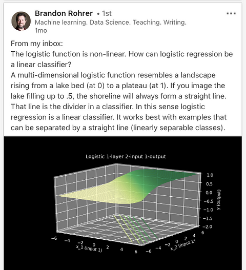
Scary looking graph that’s actual super intuitive if you stare at it long enough. From Brandon Rohrer via LinkedIn.

But back to both linear regression and logistic regression being “linear.” If we can’t come up with a line of best fit in logistic regression, where does the linear part of logistic regression come in? Well in the world of logistic regression, the outcome variable has a linear relationship with the log-odds of the independent variables.

But what in the world are the log-odds? Okay here we go….

Odds

The core of logistic regression = odds.

Intuitively, odds are something we understand —they are the probability of success to the probability of failure. In other words, they are the probability of something happening compared to the probability of something not happening.

For a concrete example of odds, we can think of a class of students. Let’s say the odds of women passing the test are 5:1, while the odds of men passing the test are 3:10. This means that, of 6 women, 5 are likely to pass the test, and that, of 13 men, 3 are likely to pass the test. The total class size here is 19 students (6 women+ 13 men).

So…aren’t odds just the same as probability?

Sadly, no! While probability measures the ratio of the number of times something happened out of the total number of times everything happened (e.g. 10 heads out 30 coin tosses), odds measures the ratio of the number of times something happened to the number of times something didn’t happen (e.g. 10 heads to 20 tails).

That means that while probability will always be confined to a scale of 0–1, odds can continuously grow from 0 to positive infinity! This presents a problem for our logistic regression model, because we know that our expected output is a probability (i.e. a number from 0–1).

So, how do we get from odds to probability?

Let’s think of a classification problem…say your favorite soccer team winning over another soccer team. You might say that the odds of your team losing are 1:6, or 0.17. And the odds of your team winning, because they’re a great team, are 6:1, or 6. You could represent those odds on a number line like below:

https://www.youtube.com/watch?v=ARfXDSkQf1Y

Now, you wouldn’t want your model to predict that your team will win on a future game just because the magnitude of the odds of them winning in the past is so much bigger than the magnitude of the odds of them losing in the past, right? There is so much more you want your model to take into account (maybe weather, maybe starting players, etc.)! So, to get the magnitude of the odds to be evenly distributed, or symmetrical, we calculate something called the log-odds.

Log-Odds

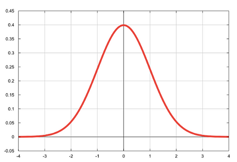
What we mean by “normally distributed”: the classic bell-shaped curve!

Log-odds is a shorthand way of referring to taking the natural logarithm of the odds. When you take the natural logarithm of something, you basically make it more normally distributed. When we make something more normally distributed, we are essentially putting it on a scale that’s super easy to work with.

When we take the log-odds, we transform the scale of our odds from 0-positive infinity to negative infinity-positive infinity. You can see this well on the bell curve above.

Even though we still need our output to be between 0–1, the symmetry we achieve by taking the log-odds gets us closer to the output we want than we were before!

Logit Function

The “logit function” is simply the math we do to get the log-odds!

Some scary math thingymabob. Er, I mean the logit function.

The logit function, graphed

The logit function puts our odds on a scale of negative infinity to positive infinity by taking their natural logarithm, as you can see above.

Sigmoid Function

Okay, but we’re still not at the point where our model is giving us a probability. Right now, all we have are numbers on a scale of negative infinity to positive infinity. Enter: the sigmoid function.

The sigmoid function, named after the s-shape it assumes when graphed, is just the inverse of the log-odds. By taking the inverse of the log-odds, we are mapping our values from negative infinity-positive infinity to 0–1. This, in turn, let’s us get probabilities, which are exactly what we want!

As opposed to the graph of the logit function where our y-values range from negative infinity to positive infinity, the graph of our sigmoid function has y-values from 0–1. Yay!

The lovely sigmoid function.

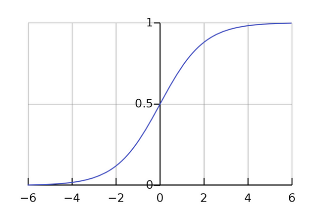
With this, we can now plug in any x-value and trace it back to its predicted y-value. That y-value will be the probability of that x-value being in one class or another.

Maximum Likelihood Estimation

…Not finished just yet.

You remember how we found the line of best fit during linear regression by minimizing the RSS (a method sometimes called the “ordinary least squares,” or OLS, method)? Here, we use something called Maximum Likelihood Estimation (MLE) to get our most accurate predictions.

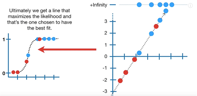
MLE gets us the most accurate predictions by determining the parameters of the probability distribution that best describe our data.

Why would we care about figuring out the distribution of our data? Because it’s cool! …But really, it just makes our data easier to work with and makes our model generalizable to lots of different data.

Logistic Regression Details, Part 2

Super generally, to get the MLE for our data, we take the data points on our s-curve and add up their log-likelihoods. Basically, we want to find the s-curve that maximizes the log-likelihood of our data. We just keep calculating the log-likelihood for every log-odds line (sort of like what we do with the RSS of each line-of-best-fit in linear regression) until we get the largest number we can.

(As an aside — we revert back to the world of natural logs because logs are the easiest form of number to work with sometimes. This is because logs are “monotonically increasing” functions, which basically just means that it consistently increases or decreases.)

The estimates that we come up with in the MLE process are those that maximize something called the “likelihood function” (which we won’t go into here).”