Now that we have covered gradient descent, linear regression, and logistic regression in Part 1, let’s get to Decision Trees and Random Forest models.
Decision Trees
A decision tree is a super simple structure we use in our heads everyday. It’s just a representation of how we make decisions, like an if-this-then-that game. First, you start with a question. Then you write out possible answers to that question and some follow-up questions, until every question has an answer.
Let’s look at a decision tree for deciding whether or not someone should play baseball on a specific day:
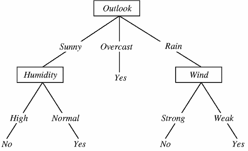
From “Machine Learning with Decision Trees” by Ramandeep Kaur
The above tree starts off with the question: what is the weather outlook today? There are three possible answers: Sunny, Overcast, or Rain.
- Let’s say it’s a sunny day: we would follow the “Sunny” branch
- The “Sunny” branch then leads us to “Humidity,” which prompts us to ask ourselves whether it’s a high-humidity day or a normal day
- Let’s say it’s a high-humidity day; we would then follow the “High” branch
- Since there are no more questions to answer at this point, we have arrived at our final decision, which is no, we should not play baseball today because it’s both sunny and very humid
And that’s really all there is to understanding decision trees!
…Just kidding. There are a few more quick things:
- Decision trees are used to model non-linear relationships (in contrast to linear regression models and logistic regression models).
- Decision trees can model both categorical and continuous outcome variables, although they are mostly used for classification tasks (i.e. for categorical outcome variables).
- Decision trees are easy to understand! You can visualize them easily and figure out exactly what’s happening at each split point. You can also see which features are most important.
- Decision trees are prone to overfitting. This is because no matter how many times you run your data through a single decision tree, since it’s just a series of if-this-then-that statements, you will always end up with the same exact outcome. This means that your decision tree will fit your training data super precisely, but that it might fail to give you useful predictions when you pass it new data.
So how does a decision tree know when to split?
(By “split” I mean to form more branches.)
There are numerous algorithms decision trees can employ, but the two most popular are ID3 (ID stands for “Iterative Dichotomizer”) and CART (CART stands for “Classification and Regression Tree”). Each of these algorithms use different measures to decide when to split. ID3 trees use information gain, while CART trees use the Gini Index.
Let’s start with ID3 trees.
ID3 Trees & Information Gain
Basically, ID3 trees are all about getting the biggest bang for their buck in the way of maximizing information gain. (Because of this, they’re also called greedy trees.)
But what is information gain? Technically speaking, information gain is a criterion that uses entropy as an impurity measure. Let’s unpack that a little bit.
Entropy
Simply, entropy is a measure of (dis)order — it tells you how much information a thing is missing, or how messy your data is. Something that is missing a lot of information is considered disordered (i.e. has a high measure of entropy), and vice versa.
Let’s look at a concrete example to solidify the intuition behind this:
Let’s say you are tasked with cleaning a messy room. On the floor are dirty clothes, maybe some dog toys, and some books strewn about. This room is extremely disordered! If we could measure its entropy, it would be super high, and its information gain would be very low. In this state, it’s pretty unworkable.
But then you see that there are some boxes in the closet, and a big Sharpie marker. You start labeling each box with the category of thing you plan to put in it. You then start cleaning up the room and placing each clothing item/dog toy/book in its respective box. You have now cleaned the room! If we could measure the room’s entropy now, it would be pretty low (and its information gain would be high). Nice job!
Similarly, ID3 trees will always make the decision that nets them the highest gain in information. More information = less entropy. This means that with every split in a decision tree the algorithm will move towards lower and lower entropy.
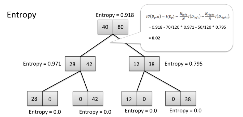
Visualizing entropy in a decision tree
In the tree above, you can see that the starting point has an entropy of 0.918, while the stopping points have entropies of 0. This tree has ended with a high information gain and a low entropy, which is exactly what we want.
(Im)Purity
In addition to moving towards low entropy, ID3 trees will also make the decision that nets them the most purity. ID3 trees do this because they want each decision to have as much clarity as possible. Something that has low entropy also has high purity. High information gain = low entropy = high purity.
This makes intuitive sense — if something is confusing and disordered (i.e. has high entropy), your understanding of that thing is murky, unclear, or impure.
CART Trees & The Gini Index
While decision trees powered by the ID3 algorithm aim to maximizeinformation gain at each split, decision trees using the CART algorithm aim to minimize a measure called the Gini Index.
The Gini Index basically tells you how often a randomly chosen data point from your dataset is likely to be mis-categorized. In CART trees (and in life), we always want to minimize the likelihood of incorrectly labeling any part of our data. It’s really as simple as that!
Okay that all makes some sense, but what about the non-linear stuff you mentioned before?
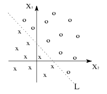
Visualization of linearly-separable data
In Part 1 of this series we learned that linear relationships are defined by lines.
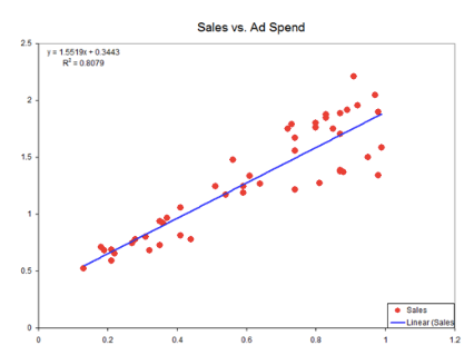
Visualization of linear function underlying a linear model.
Basically, we know our data has linearity of some sort when we can separate our data points into groups by using a line (or linear plane), like in the top-most graph.
Similarly, we know a model is linear when we can graph the relationship between variables with some sort of line. This line is a visualization of the linear function that undergirds a linear model, like the blue line on the second graph above.
Non-linearity is really just the opposite of this. You can think of non-linear data and functions in a few different ways:
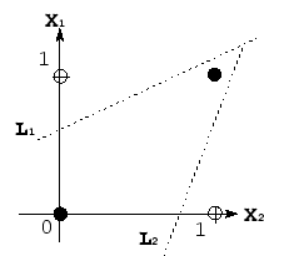
Visualization of non-linearly-separable data
- With non-linear data, you will not be able to visualize a linear plane that segments your data. When you cannot separate your data linearly, your model is reliant on a non-linear function. This, in turn, means that your model is non-linear!
- While linear functions have a constant slope (because a small change in x results in the same small change in y), non-linear functions do not. Their slope might instead grow exponentially, for instance.
- You can also use the same analogy as we did in Part 1, but instead of a small change in your independent variable(s) resulting in the same small change in your dependent variable, a small change in your independent variable(s) will results in a huge change, or a super small change, in your dependent variable when your working with non-linear functions.
Decision trees are great at modeling non-linear relationships because they don’t rely on a linear plane to separate the data. (While that sentence might sound scary, it’s really not — we know intuitively that decision trees don’t linearly separate data. You can prove this to yourself by simply looking at our tree structure! How would you group all the “yes”s into 1 area and all the “no”s into another area only using a line? You can’t!)
…Okay and now what about the overfitting stuff?
So, yes, decision trees (regardless of which algorithm they use) are great when you want to do exploratory analysis. They excel at outlining the important features in your data and allowing you to see how each feature interacts. However, they tend to overfit your data. In turn, this means that decision trees are not great at predicting or classifying data they haven’t seen before.
To combat this overfitting, data scientists have come up with models called ensemble models. These models basically just lump many decision trees together and use their collective power to make a prediction that can withstand rigorous testing.
Enter: Random Forest
Random Forest is arguably the most popular ensemble model for beginner data scientists.
https://cdn.firespring.com/images/442c053c-745c-4bf3-b4a2-21b6fa79ddca.jpg
Ensemble, you say?
So, an ensemble model is just an ensemble of many models grouped other, as we said above.
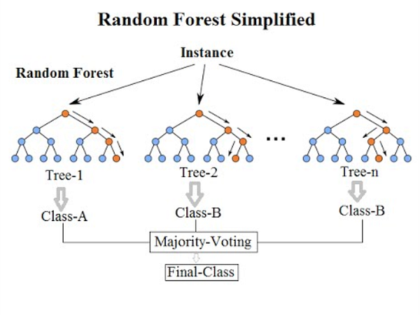
(Sorry for the blurriness, but I just love this image.) Random Forest structure from KDNuggets.
As you can see in the diagram to the left, an ensemble model like Random Forest is just a bunch of decision trees. Here, you can see that there are 3 decision trees.
Ensemble models like Random Forest are designed to decrease overfitting and variance by using bagging algorithms.
We know that decision trees are prone to overfitting. In other words, a single decision tree can be wonderful at finding a solution for a specific problem, but quite crappy if applied to a problem it’s never seen before. Similar to the adage “two heads are better than one,” ensemble models use many decision trees that are good at their particular task to make a larger model that’s great at many different tasks. Think of it this way — are you more likely to make a good business decision by listening to the advice of a single employee or many employees who bring a diversity of experience with them? Probably the latter. More decision trees = less overfitting.
Okay, I get overfitting, but what’s this variance you’re talking about?
In the data science world, we have to combat against more than just overfitting. We have to also fight back against something called variance.

A model with “high variance” is a model whose outcome can vary if its inputs are changed even the tiniest bit. Much like overfitting, this means that models with high variance do not generalize well to new data.
I like to think of variance in terms of physical balance: if you are balancing on one foot while standing on solid ground you’re not likely to fall over. But what if there are suddenly 100 mph wind gusts? I bet you’d fall over. That’s because your ability to balance on one leg is highly dependent on the factors in your environment. If even one thing changes, it could completely mess you up! This is how it is when models have high variance. If we mess with any factors in its training data, we could completely change the outcome. This is not stable, and therefore not a model off of which we’d want to make decisions.
Bagging Algorithms
Before we dive into bagging algorithms, on which Random Forest relies heavily, there’s one thing we still need to cover, and that is the idea of learners.
In machine learning, there are weak learners and strong learners, and bagging algorithms (or “Bootstrap AGGregatING” algorithms) deal with weak learners.
(We won’t get into strong learners here, but keep an eye out for them in future parts of this series!)
Weak Learners
Weak learners make up the backbone of Random Forest models.
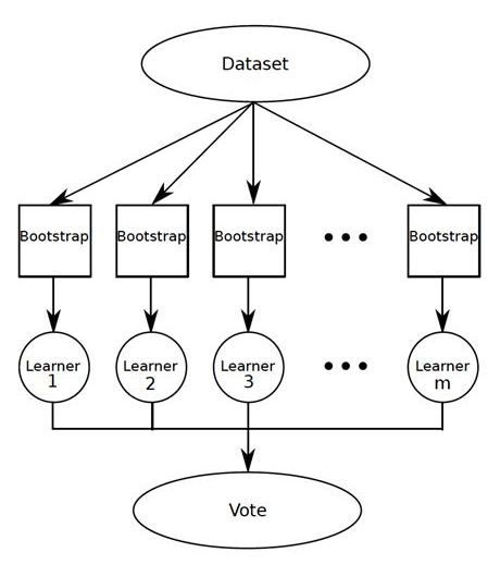
The bottom row of this ensemble model (let’s call it a Random Forest) is where our “weak learners” live!
Simply put, weak learners are algorithms that predict/classify data with an accuracy (or other evaluation metric) slightly better than chance. The reason these guys are useful is that we can pool them together to make a larger model whose predictions/classifications are super good!
…Okay, Back to Bagging
Ensemble models like Random Forest use bagging algorithms to escape the pitfalls of high variance and overfitting to which simpler models, such as individual decision trees, are prone.

Bagging algorithms’ super power is that they work with random samples of your data with replacement.
This basically just means that, as the algorithm goes through and builds decision trees with random samples of your data, there are no data points that it can’t use. For example, just because 1 decision tree is being made with 20 data points doesn’t mean that another decision tree can’t also be made using 12 of those same 20 data points. Yay, probability!
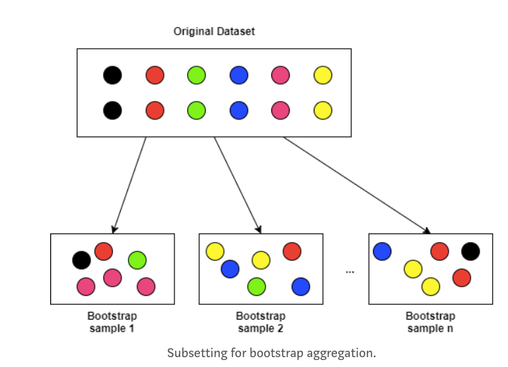
From Decision Trees and Random Forests for Classification and Regression pt.2, by Haihan Lan
A cool thing about Random Forest models is that they can do all this random sampling-with-replacement for every decision tree simultaneously (or in “parallel”). And because we are in the world of random-sampling-with-replacement, we can also assume that each of our decision trees is independent from the other.
In summary: Random Forest models use bagging algorithms to build little decision trees, each one of which is built simultaneously with random subsets of your data.
…But There’s More!
Not only does each tree in a Random Forest model only contain a subset of your data, each tree also only uses a subset of features (i.e. columns) from your data.
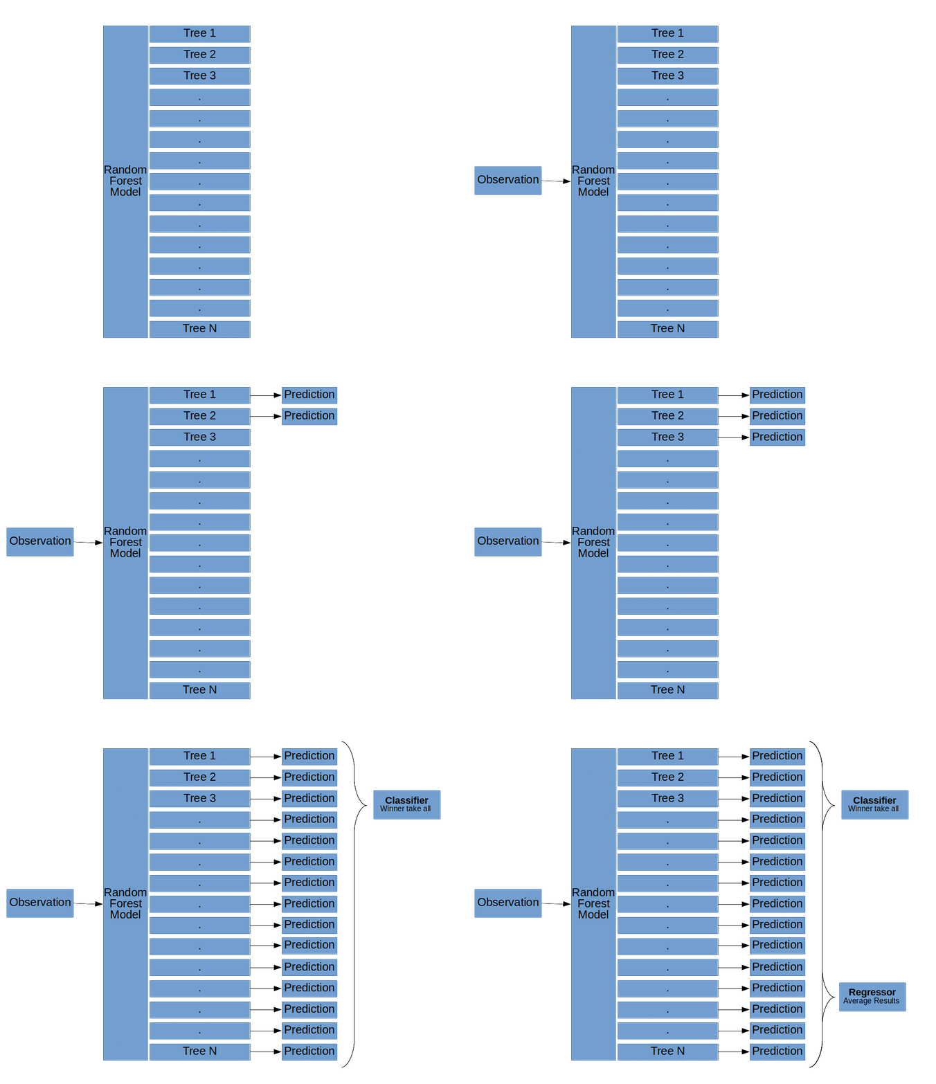
The basic structure of a Random Forest model (Random Forests, Decision Trees, and Ensemble Methods Explained, by Dylan Storey)
For instance, let’s say we are trying to classify a book as sold or unsold based on author, publication date, number of pages, and language. And we have 10,000 books in our dataset. In a Random Forest model, not only would each of our decision trees only use a random sample of the 10,000 books, each decision tree would also only use a random sample of the features: perhaps one decision tree would use author and publication date, while another decision tree would use author and number of pages. And yet another decision tree could use language and publication date. The point of this is that when we average the predictions of all of these decision trees (i.e. “weak learners) together, we get a super robust prediction!
And that is pretty much it! When we are using Random Forest models for classification, we take the majority vote of all the decision trees and use that as the outcome. When we are using Random Forest models for regression, we average all the probabilities from each decision tree and use that number as an outcome.
Through this post we learned all about decision trees, non-linearity, overfitting and variance, and ensemble models like Random Forest. Keep an eye out for Part 3 — we’ll be covering two linear models that are a bit more advanced than what we covered in Part 1: SVM and Naive Bayes.


