After presenting in two previous posts ( post 1, post 2) the factors that have contributed to unleashing the potential of Artificial Intelligence and related technologies as Deep Learning, now is time to start to review the basic concepts of neural networks.
In the same way that when you start programming in a new language there is a tradition of doing it with a Hello World print, in Deep Learning you start by creating a recognition model of handwritten numbers. Through this example, this post will present some basic concepts of neural networks, reducing theoretical concepts as much as possible, with the aim of offering the reader a global view of a specific case to facilitate the reading of the subsequent posts where different topics in the area will be dealt with in more detail.
Case of study: digit recognition
In this section, we introduce the data we will use for our first example of neural networks: the MNIST dataset, which contains images of handwritten digits.
The MNIST dataset, which can be downloaded from The MNIST databasepage[1], is made up of images of hand-made digits. This dataset contains 60,000 elements to train the model and 10,000 additional elements to test it, and it is ideal for entering pattern recognition techniques for the first time without having to spend much time preprocessing and formatting data, both very important and expensive steps in the analysis of data and of special complexity when working with images; this dataset only requires small changes that we will comment on below.
This dataset of black and white images has been normalized to 20×20 pixels while retaining their aspect ratio. In this case, it is important to note that the images contain gray levels as a result of the anti-aliasing[2] technique, used in the normalization algorithm (reducing the resolution of all images to one of lower). Subsequently, the images were centered on a 28×28 pixel, calculating the center of mass of these and moving the image in order to position this point in the center of the 28×28 field. The images are of the following style:

Pixel images of handwritten texts ( From: MNIST For ML Beginners, tensorflow.org)
Furthermore, the dataset has a label for each of the images that indicates what digit it represents, being, therefore, a supervised learning which we will discuss in this chapter.
This input image is represented in a matrix with the intensities of each of the 28×28 pixels with values between [0, 255]. For example, this image (the eighth of the training set)
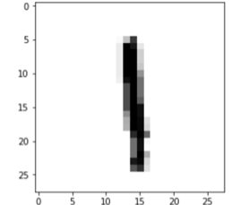
It is represented with this matrix of 28×28 points (the reader can check it in the notebook of this chapter):
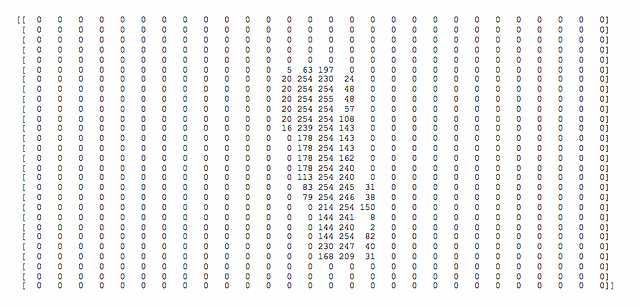
On the other hand, remember that we have the labels, which in our case are numbers between 0 and 9 that indicate which digit the image represents, that is, to which class it is associated. In this example, we will represent each label with a vector of 10 positions, where the position corresponding to the digit that represents the image contains a 1 and the rest contains 0s. This process of transforming the labels into a vector of as many zeros as the number of different labels, and putting a 1 in the index corresponding to the label, is known as one-hot encoding.
Perceptron
Before moving forward, a brief intuitive explanation of how a single neuron works to fulfill its purpose of learning from the training dataset can be helpful for the reader. Let’s look at a very simple example to illustrate how an artificial neuron can learn.
Regression algorithms
Based on what has been explained in the previous chapter, let us make a brief reminder about classic Machine Learning regression and classification algorithms since they are the starting point of our Deep Learning explanations.
We could say that regression algorithms model the relationship between different input variables (features) using a measure of error, the loss, which will be minimized in an iterative process in order to make predictions “as accurate as possible”. We will talk about two types: logistic regression and linear regression.
The main difference between logistic and linear regression is in the type of output of the models; when our output is discrete, we talk about logistic regression, and when the output is continuous we talk about linear regression.
Following the definitions introduced in the first chapter, logistic regression is an algorithm with supervised learning and is used to classify. The example that we will use next, which consists of identifying which class each input example belongs to by assigning a discrete value of type 0 or 1, is a binary classification.
A plain artificial neuron
In order to show how a basic neuronal is, let’s suppose a simple example where we have a set of points in a two-dimensional plane and each point is already labeled “square” or “circle”:
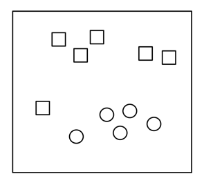
Given a new point “X“, we want to know what label corresponds to it:
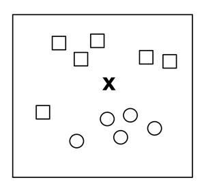
A common approach is to draw a line that separates the two groups and use this line as a classifier:
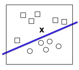
In this case, the input data will be represented by vectors of the form (x1, x2) that indicate their coordinates in this two-dimensional space, and our function will return ‘0’ or ‘1’ (above or below the line) to know if it should be classified as “square” or “circle”. As we have seen, it is a case of linear regression, where “the line” (the classifier) following the notation presented in chapter 1 can be defined by:

More generally, we can express the line as:

To classify input elements X, which in our case are two-dimensional, we must learn a vector of weight W of the same dimension as the input vectors, that is, the vector (w1, w2) and a b bias.
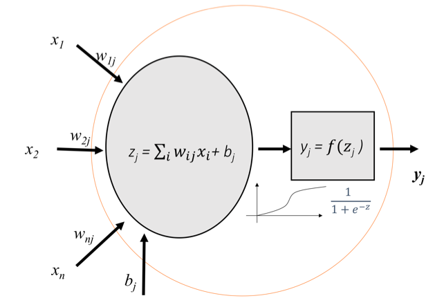
With these calculated values, we can now construct an artificial neuron to classify a new element X. Basically, the neuron applies this vector W of calculated weights on the values in each dimension of the input element X, and at the end adds the bias b. The result of this will be passed through a non-linear “activation” function to produce a result of ‘0’ or ‘1’. The function of this artificial neuron that we have just defined can be expressed in a more formal way such as:

Now, we will need a function that applies a transformation to variable z so that it becomes ‘0’ or ‘1’. Although there are several functions (which we will call “activation functions” as we will see in chapter 4), for this example we will use one known as a sigmoid[3] function that returns an actual output value between 0 and 1 for any input value:

If we analyze the previous formula, we can see that it always tends to give values close to 0 or 1. If the input z is reasonably large and positive, “e” at minus z is zero and, therefore, the y takes the value of 1. If z has a large and negative value, it turns out that for “e” raised to a large positive number, the denominator of the formula will turn out to be a large number and therefore the value of y will be close to 0. Graphically, the sigmoid function presents this form:
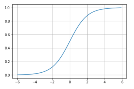
So far we have presented how to define an artificial neuron, the simplest architecture that a neural network can have. In particular this architecture is named in the literature of the subject as Perceptron[4] (also called linear threshold unit (LTU)), invented in 1957 by Frank Rosenblatt, and visually summarized in a general way with the following scheme:
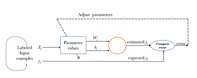
Finally, let me help the reader to intuit how this neuron can learn the weights W and the biases b from the input data that we already have labeled as “squares” or “circles” (in chapter 4 we will present how this process is done in a more formal way).
It is an iterative process for all the known labeled input examples, comparing the value of its label estimated through the model, with the expected value of the label of each element. After each iteration, the parameter values are adjusted in such a way that the error obtained is getting smaller as we keep on iterating with the goal of minimizing the loss function mentioned above. The following scheme wants to visually summarize the learning process of one perceptron in a general way:
Multi-Layer Perceptron
But before moving forward with the example, we will briefly introduce the form that neural networks usually take when they are constructed from perceptrons like the one we have just presented.
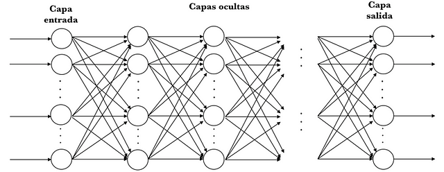
In the literature of the area we refer to a Multi-Layer Perceptron (MLP) when we find neural networks that have an input layer, one or more layers composed of perceptrons, called hidden layers and a final layer with several perceptrons called the output layer. In general we refer to Deep Learning when the model based on neural networks is composed of multiple hidden layers. Visually it can be presented with the following scheme:
MLPs are often used for classification, and specifically when classes are exclusive, as in the case of the classification of digit images (in classes from 0 to 9). In this case, the output layer returns the probability of belonging to each one of the classes, thanks to a function called softmax. Visually we could represent it in the following way:
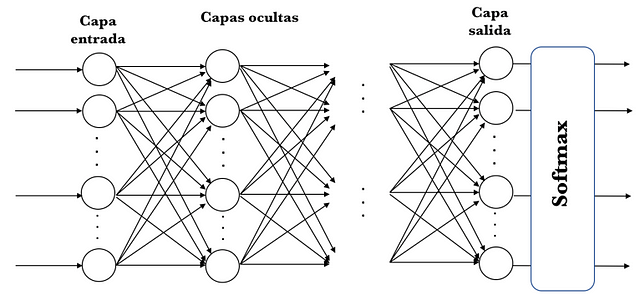
As we will present in chapter 4, there are several activation functions in addition to the sigmoid, each with different properties. One of them is the one we just mentioned, the softmax activation function[5], which will be useful to present an example of a simple neural network to classify in more than two classes. For the moment we can consider the softmax function as a generalization of the sigmoid function that allows us to classify more than two classes.
Softmax activation function
We will solve the problem in a way that, given an input image, we will obtain the probabilities that it is each of the 10 possible digits. In this way, we will have a model that, for example, could predict a nine in an image, but only being sure in 80% that it is a nine. Due to the stroke of the bottom of the number in this image, it seems that it could become an eight in a 5% chance and it could even give a certain probability to any other number. Although in this particular case we will consider that the prediction of our model is a nine since it is the one with the highest probability, this approach of using a probability distribution can give us a better idea of how confident we are of our prediction. This is good in this case, where the numbers are made by hand, and surely in many of them, we cannot recognize the digits with 100% certainty.
Therefore, for this example of MNIST classification we will obtain, for each input example, an output vector with the probability distribution over a set of mutually exclusive labels. That is, a vector of 10 probabilities each corresponding to a digit and also the sum of all these 10 probabilities results in the value of 1 (the probabilities will be expressed between 0 and 1).
As we have already advanced, this is achieved through the use of an output layer in our neural network with the softmax activation function, in which each neuron in this softmax layer depends on the outputs of all the other neurons in the layer, since that the sum of the output of all of them must be 1.
But how does the softmax activation function work? The softmax function is based on calculating “the evidence” that a certain image belongs to a particular class and then these evidences are converted into probabilities that it belongs to each of the possible classes.
An approach to measure the evidence that a certain image belongs to a particular class is to make a weighted sum of the evidence of belonging to each of its pixels to that class. To explain the idea I will use a visual example.
Let’s suppose that we already have the model learned for the number zero (we will see later how these models are learned). For the moment, we can consider a model as “something” that contains information to know if a number is of a certain class. In this case, for the number zero, suppose we have a model like the one presented below:
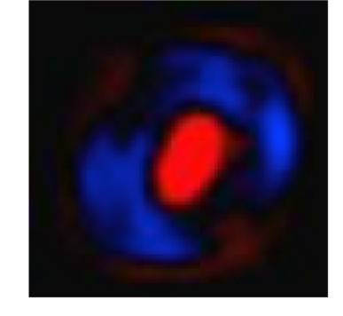
Source: Tensorflow tutorial[6])
In this case, with a matrix of 28×28 pixels, where the pixels in red (in the white/black edition of the book is the lightest gray) represent negative weights (i.e., reduce the evidence that it belongs), while that the pixels in blue (in the black/white edition of the book is the darkest gray) represent positive weights (the evidence of which is greater increases). The black color represents the neutral value.
Let’s imagine that we trace a zero over it. In general, the trace of our zero would fall on the blue zone (remember that we are talking about images that have been normalized to 20×20 pixels and later centered on a 28×28 image). It is quite evident that if our stroke goes over the red zone, it is most likely that we are not writing a zero; therefore, using a metric based on adding if we pass through the blue zone and subtracting if we pass through the red zone seems reasonable.
To confirm that it is a good metric, let’s imagine now that we draw a three; it is clear that the red zone of the center of the previous model that we used for the zero will penalize the aforementioned metric since, as we can see in the left part of this figure, when writing a three we pass over:
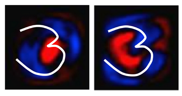
Source: Tensorflow tutorial[6])
But on the other hand, if the reference model is the one corresponding to number 3 as shown in the right part of the previous figure, we can see that, in general, the different possible traces that represent a three are mostly maintained in the blue zone.
I hope that the reader, seeing this visual example, already intuits how the approximation of the weights indicated above allows us to estimate what number it is.
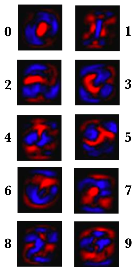
Source: Tensorflow tutorial[6])
The previous figure shows the weights of a concrete model example learned for each of these ten MNIST classes. Remember that we have chosen red (lighter gray in black and white book edition) in this visual representation for negative weights, while we will use blue to represent positives.
Once the evidence of belonging to each of the 10 classes has been calculated, these must be converted into probabilities whose sum of all their components add 1. For this, softmax uses the exponential value of the calculated evidence and then normalizes them so that the sum equates to one, forming a probability distribution. The probability of belonging to class i is:

Intuitively, the effect obtained with the use of exponentials is that one more unit of evidence has a multiplier effect and one unit less has the inverse effect. The interesting thing about this function is that a good prediction will have a single entry in the vector with a value close to 1, while the remaining entries will be close to 0. In a weak prediction, there will be several possible labels, which will have more or less the same probability.
REFERENCES
[1] The MNIST database of handwritten digits. [en línea]. Available at: http://yann.lecun.com/exdb/mnist [Consulta: 24/02/2017].
[2] Wikipedia, (2016). Antialiasing [en línea]. Available at: https://es.wikipedia.org/wiki/Antialiasing [Visited: 9/01/2016].
[3] Wikipedia, (2018). Sigmoid function [en línea]. Available at: https://en.wikipedia.org/wiki/Sigmoid_function [Visited: 2/03/2018].
[4] Wikipedia (2018). Perceptron [en línea]. Available at https://en.wikipedia.org/wiki/Perceptron [Visited 22/12/2018]
[5] Wikipedia, (2018). Softmax function [en línea]. Available at: https://en.wikipedia.org/wiki/Softmax_function [Visited: 22/02/2018].
[6] TensorFlow, (2016) Tutorial MNIST beginners. [en línea]. Available at: https://www.tensorflow.org/versions/r0.12/tutorials/mnist/beginners/[Visited: 16/02/2018].


