Physics-guided Neural Networks (PGNNs)

Physics-based models are at the heart of today’s technology and science. Over recent years, data-driven models started providing an alternative approach and outperformed physics-driven models in many tasks. Even so, they are data hungry, their inferences could be hard to explain and generalization remains to be a challenge. Combining data and physics could reveal the best of both worlds.

When machine learning algorithms are learning, they are actually searching for a solution in the hypothesis space you defined by your choice of algorithm, architecture, and configuration. Hypothesis space could be quite large even for a fairly simple algorithm. Data is the only guide we use to look for a solution in this huge space. What if we can use our knowledge of the world — for example, physics— together with data to guide this search?

This is what Karpatne et al. explained in their paper Physics-guided Neural Networks (PGNN): An Application in Lake Temperature Modeling. In this post, I will explain why this idea is crucial and I will also describe how they did it by summarizing the paper.

Imagine you have sent your alien 👽 friend (optimization algorithm) to a supermarket (hypothesis space) to buy your favorite cheese (solution). The only clue she has is the picture of the cheese (data) you gave her. Since she lacks the preconceptions we have about supermarkets she will have a hard time finding the cheese. She might wander around cosmetics, cleaning supplies before even reaching the food section.

Finally reached the food section (courtesy of Dominic L. Garcia).

This is similar to how machine learning optimization algorithms like gradient descent look for a hypothesis. Data is the only guide. Ideally, this should work just fine but most of the time the data is noisy or not enough. Incorporating our knowledge into the optimization algorithms — search for the cheese in the food section, don’t even look at the cosmetics — could alleviate these challenges. Let’s see next, how we can actually do this.

How to guide an ML algorithm with physics

Now, let me summarize how the authors utilize physics to guide a machine learning model. They present two approaches for this: (1) using physics theory, they calculate additional features (feature engineering) to feed into the model along with the measurements and (2) they add a physical inconsistency term to the loss function in order to punish physically inconsistent predictions.

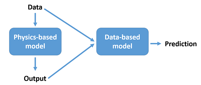
 (1) Feature engineering using a physics-based model

(2) Data + Physics driven loss function

The first approach, feature engineering, is extensively used in machine learning. The second approach, however, is compelling. Very much like adding a regularization term to punish overfitting, they add a physical inconsistency term to the loss function. Hence, with this new term, the optimization algorithm should also take care of minimizing physically inconsistent results.

In the paper, Karpatne et al. combined these two approaches with a neural network and demonstrated an algorithm they call physics-guided neural network (PGNN). There are two main advantages PGNNs could provide:

• Achieving generalization is a fundamental challenge in machine learning. Since physics models, mostly, do not depend on data, they might perform well on unseen data, even from a different distribution.
• Machine learning models are sometimes referred to as black-box models due to the fact that it is not always clear how a model reaches a specific decision. There is quite a lot of work going into Explainable AI (XAI) to improve model interpretability. PGNNs could provide a basis towards XAI as they present physically consistent and interpretable results.

Application example: Lake temperature modeling

In the paper, lake temperature modeling is given as an example to demonstrate the effectiveness of the PGNN. Water temperature controls the growth, survival, and reproduction of biological species living in the lake. Therefore accurate observations and predictions of temperature are crucial for understanding the changes occurring in the community. The task is to develop a model that can predict the water temperature as a function of depth and time, for a given lake. Now let’s see how they applied (1) feature engineering and (2) loss function modification for this problem.

(1) For feature engineering, they used a model called the general lake model (GLM) to generate new features and feed them into the NN. It is a physics-based model that captures the processes governing the dynamics of temperature in a lake (heating due to sun, evaporation etc.).

(2) Let’s now see how they defined this physical inconsistency term. It is known that denser water sinks. The relationship between water temperature and its density is also known. Hence predictions should follow the fact that the deeper the point, the higher the predicted density. If for a pair of points, the model predicts higher density for the point closer to the surface, this is a physically inconsistent prediction.

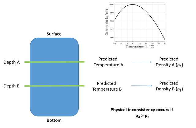
Now it is possible to incorporate this idea into the loss function. We would like to punish if ρA> ρB and do nothing otherwise. Moreover, for a larger inconsistency, the punishment should be higher. This can be done easily by adding the value of the function max( ρA- ρB, 0) to the loss function. If ρA> ρB (i.e. inconsistency), the function will give a positive value that will increase the value of the loss function (the function we are trying to minimize), otherwise it will give zero leaving the loss function unchanged.

At this point, two modifications are necessary to the function in order to use it properly. What is important is the average inconsistency of all the pairs, not one single pair. Therefore it is possible to sum max( ρA- ρB, 0) for all points and divide by the number of points. Also, it is critical to control the relative importance of minimizing physical inconsistency. This can be done by multiplying the average physical inconsistency with a hyperparameter (works like the regularization parameter).

 Physical inconsistency term of the loss function

Results

Here are the results of 4 models. They are:

• PHY: General lake model (GLM).
• NN: A neural network.
• PGNN0: A neural network with feature engineering. Results of the GLM are fed into the NN as additional features.
• PGNN: NN with feature engineering and with the modified loss function.

And two metrics for evaluation:

• RMSE: Root mean square error.
• Physical Inconsistency: Fraction of time-steps where the model makes physically inconsistent predictions.

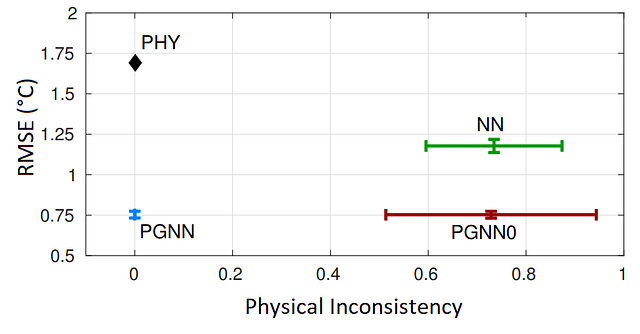
Results on Lake Mille Lacs

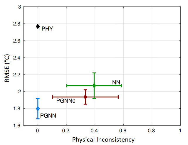
        Results on Lake Mendota

Comparing NN with the PHY we can conclude that NN gives more accurate predictions at the expense of physically inconsistent results. Comparing PGNN0 and PGNN we can see that physical inconsistency is eliminated mostly thanks to the modified loss function. Improved accuracy is mostly due to feature engineering with some contribution from the loss function.

To sum things up, these first results show us that this new type of algorithm, PGNN, is very promising for providing accurate and physically consistent results. Moreover, incorporating our knowledge of the world into the loss function provides an elegant way to improve the generalization performance of machine learning models. This seemingly simple idea has the potential to fundamentally improve the way we conduct machine learning and scientific research.