TLDR, models always take the route of least effort.
Training machine learning models is far from easy. In fact, the unaware data scientist might trip and fall in as many pitfalls as there are living AWS instances. The list is endless but divides itself nicely into two broad categories: underfitting, your model is bad, and overfitting, your model is still bad, but you think it isn’t. While overfitting can manifest itself in various ways, shortcut learning is a recurring flavor when dealing with custom datasets and novel problems. It affected me; it might be affecting you.
Informally, shortcut learning occurs whenever a model fits a problem on data not expected to be relevant or present, in general.
A practical example is a dog/cat classifier that, instead of properly recognizing dog- and cat-features, specializes in detecting leashes. Assuming leashes means dogs will likely do well most of the time, but leashes are not a general descriptor of dogness. That’s lazy work!
In other words, the model took a shortcut to solve the problem. It cheated.
Shortcut learning typically arises when there isn’t enough data to force algorithms into learning the task properly. In our dog/cat example, most dog pictures likely included a leash while cat pictures didn’t. Learning to detect leashes is a far simpler task than recognizing pets: they are simple, they contrast with the dog, and they are usually vibrant colored.
The catch is that machine learning algorithms favor the route of least effort.
Putting it another way, a machine learning algorithm will only learn what you want if that is the easiest thing it can do to maximize its metrics. As long as there are leash-like shortcuts, models will cheat.

Shortcut learning helps us realize that we don’t give algorithms any real, meaningful instruction on what to learn. We can’t blame our tools for slacking — they just fit data, after all.
From the above, it follows that we don’t have any reliable way to teach algorithms how to tell background from the foreground. If all dog pictures were outdoor and all cat ones were indoor, it wouldn’t surprise me to see classifiers becoming experts at detecting sky and grass — not dogs and cats.
These small observations carry a profound insight into machine learning’s current nature: it is still a highly random process.
To this date, the only sure-fire way to reduce the likelihood of shortcuts in your data is to… add more data!
If we increase our dogs and cats dataset to include outdoor and indoor pictures of each kind and leash-less dogs and leashed cats, we might get a step closer to a true dog and cat classifier. We might get. There is no guarantee there aren’t any other shortcuts lingering around — you never know.
Removing shortcuts is much harder than it seems. It is quite challenging to disentangle concepts by simply adding contrasting data. For instance, most cars are found outdoors; however, a car is a car regardless of its location. If we blindly search for car images, we are bound to get shortcuts such as road = car, asphalt = car, tire = car, etc.
To better illustrate this, consider this simple custom dataset:
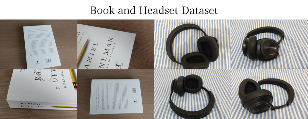
This eight-images dataset shows a single book and a single headset. While no one in their right mind would even consider this to be a proper dataset, let’s give it the benefit of the doubt and wonder how a model would fit it.
The book images have many straight lines, lots of white, lots of brown, and text, while the headset images have lots of blue, stripes, black, and curves. A model trained on such data would promptly classify any black book as a headset and any brown thing as a book. A CNN, in particular, would quickly fit local patterns such as text = books and stripes = headset.
How can we solve this? More data!
After some coding, we got ourselves a Google Images crawler and downloaded a thousand book images and a thousand headset images. Let’s inspect what Google has to offer regarding books and headsets:


What we got is that most book images are of book stacks or bookshelves, which, by the way, are quite likely to be made of wood, and all headset images come from shopping sites; these are all illustrations, not real images. If we scroll down (a lot), we get pictures of people wearing headsets, opening an avenue for the algorithm to mistake faces for headsets.
In other words, blindly pouring data only made our problem worse.
While all datasets mentioned so far are toy problems, these shortcut issues are more common than we would like to acknowledge. Shortcuts are especially frequent when constructing custom datasets, which is what many people do. Such datasets are typically small and contain data coming from only a handful of sources or were generated by just a couple of hardworking people.
A practical example is AI applied to medicine. Building a medical imaging dataset is quite expensive, as you need everyone’s permission, only doctors can label it, and some conditions are naturally rare. On top of that, images are of high resolution, and their content can be quite complex. It is rather easy for models to fit arbitrary structures instead of learning their intended task. Some images also contain metadata, such as the patient name, hospital logo, and time of day, all of which can become nasty shortcuts.
Custom datasets involving humans, in particular, are quite prone to such issues as well. In many, there is a limited budget for actors and scenes, leading to poor variety. This setup is quite open for algorithms to overfit to specific actors or clothing elements rather than what they are doing.
To better understand this phenomenon, we need a bit of formality…
Classification is a mapping from some data x to a set of labels y, or x → y. For instance, if we want to detect persons in pictures, x are pictures, and y is whether they have a person or not. In this framework, a classifier is a function that, given an x, answers its y. A good classifier will answer the right label most of the time; a bad classifier won’t.
Without any loss of generality, we might breakdown our x elements as a “signal,” which is the real thing we want to track, and a set of “noises” that tarnish it. Thus, x can be rewritten as s + n₁ + n₂ + n₃ + …
In our original example, the signals are the dogs and cats, the things we really want to track, and the noises are everything else: the leashes, the background elements, the pet color, their pose, etc. By themselves, these noisy elements are harmless. Shortcut learning arises when these are simultaneously easily detectable and correlated with y. Thus, detecting the noise becomes the route of least effort — the shortcut.
This gets worse with powerful models, such as neural networks and support vector machines. These models’ flexibility might backfire into learning non-trivial couplings of noises, such as “leash or outdoor equals dog” and “raised tail equals cat.” Never underestimate a model’s ability to overfit.
It is important to mention that our signal itself is also not a single beacon. Many pet breeds vary in color, and owners might style their pets to their hearts’ content. A classifier might fit some of these signals, but not all — or jointly fit both noise and signal elements.

Apowerful concept in this analysis is the signal-to-noise-ratio. As we add more images, some noises cancel out. For instance, as we added unleashed dogs to our data, detecting leashes became increasingly less rewarding. The more data we add, the less noise we get, and, gradually, our signal shall become the only reliable source for classification.
At this point, we are ready to talk about addressing shortcut learning. Without changing the problem, there are a couple of ways in which we can alleviate it:
- Add lots of data: as discussed, one effective way of raising the signal-to-noise-ratio is pouring more data, evening out the noise. For simple domains, however, blindly adding data might work against you. A safer alternative is to…
- Add the right data: when it’s expensive to find quality data, it helps to locate current shortcuts and aim for opposing data. In our example, that means searching for leashed cats and unconstrained dogs.
- Include regularization: techniques such as dropout and weight decay aim at making the learning task artificially harder, forcing the algorithm to rely on robust signals rather than occasional hints. Similarly, you might…
- Use smaller, dumber models: tiny models cannot focus on as many properties as bigger ones; therefore, they are less prone to rely on spurious correlations and more likely to pay attention to the true signal.
In this regard, it is imperative to highlight that data augmentation is not an effective measure to address shortcut learning. The reason being that most operations are likely to either preserve or augment pre-existing shortcuts. A leash is still a leash even if flipped, rotated, zoomed, sheared, and hue-shifted. Cutout might help to some extent, but I wouldn’t rely on it.
If you are able to change the problem formulation, an effective way of avoiding shortcuts almost entirely is recasting classification as detection or segmentation. In these more advanced formulations, you are explicitly telling the algorithm what to look for and requiring it to show its findings. While this approach effectively solves shortcut learning, annotating your existing data might prove to be prohibitive in most cases.

One aspect we haven’t discussed so far is how to spot shortcut learning. This is a tricky subject, as with detecting any form of overfitting; however, we can take some specific actions to uncover shortcuts or at least find evidence that something is wrong.
The direct approach is to run interpretability models. These algorithms try to explain which features of your data contribute the most to the models’ outputs. Many of these techniques are model agnostic, meaning that they can be applied regardless of the model used, such as the SHAP technique.
In the case of vision models, most interpretation tools highlight the specific areas that contributed the most to a specific answer. It takes some time to inspect all images, but it certainly pays off. You should look for the obvious: the area that contributes to “dog” should be the dog itself or some of its dog-features, such as its face, ears, and feet.
Occasional exceptions are OK, but you should move them to a separate folder for a second look. Inspecting all odd detections together might reveal interesting patterns that you wouldn’t otherwise spot. I also recommend sorting your data by loss. You are bound to find odd entries and badly labeled data at both the low-loss and high-loss ends.
If you don’t want to go through all this trouble, there are some automated ways of checking if something is odd. These methods won’t generally tell you what is wrong but are sure to raise some eye browns if something is awry.
A quick assessment is swapping your training/test split. If you train-on-test and test-on-train, not much should change, apart from somewhat inferior results. If results are significantly lower (or higher!) or the training progresses at a particularly different pace, something might be off.
A more robust assessment is cross-validation. The general idea is to create several training-test splits out of the same dataset and train a model for each. In normal circumstances, all models should reach similar performance levels. If that’s not the case, your model is not truly generalizing to unseen data.
Inthis article, we overviewed what shortcut learning is, why it is so hard to get rid of it, a couple of measures we can take to handle it, and, finally, how we can search for them directly and indirectly. If you are working with custom, in-house, datasets, I highly encourage you to go through some of the outlined steps and see if your models are really fitting to the intended signals and, if they aren’t, uncover what they are really fitting to.
Throughout this piece, I focused on image classification. However, this is not strictly a vision issue. There can be shortcuts on text, graphs, and audio as well. Similar issues also arise in regression and reinforcement scenarios.
I hope this has been a pleasant read for you as it was for me to write. If you would like to read more on the topic, I highly recommend the recent work of Geirhos et al. You can find it here.
Thanks for reading


