TL;DR: One of the challenges that have so far precluded the wide adoption of graph neural networks in industrial applications is the difficulty to scale them to large graphs such as the Twitter follow graph. The interdependence between nodes makes the decomposition of the loss function into individual nodes’ contributions challenging. In this post, we describe a simple graph neural network architecture developed at Twitter that can work on very large graphs.
This post was co-authored with Fabrizo Frasca and Emanuele Rossi.
Graph Neural Networks (GNNs) are a class of ML models that have emerged in recent years for learning on graph-structured data. GNNs have been successfully applied to model systems of relation and interactions in a variety of different domains, including social science, computer vision and graphics, particle physics, chemistry, and medicine. Until recently, most of the research in the field has focused on developing new GNN models and testing them on small graphs (with Cora, a citation network containing only about 5K nodes, still being widely used [1]); relatively little effort has been invested in dealing with large-scale applications. On the other hand, industrial problems often deal with giant graphs, such as Twitter or Facebook social networks containing hundreds of millions of nodes and billions of edges. A big part of methods described in the literature are unsuitable for these settings.
In a nutshell, graph neural networks operate by aggregating the features from local neighbour nodes. Arranging the d-dimensional node features into an n×d matrix X (here n denotes the number of nodes), the simplest convolution-like operation on graphs implemented in the popular GCN model [2] combines node-wise transformations with feature diffusion across adjacent nodes
Y = ReLU(AXW).
Here W is a learnable matrix shared across all nodes and A is a linear diffusion operator amounting to a weighted average of features in a neighbourhood [3]. Multiple layers of this form can be applied in sequence like in traditional CNNs. Graph neural networks can be designed to make predictions at the level of nodes (e.g. for applications such as detecting malicious users in a social network), edges (e.g. for link prediction, a typical scenario in recommender systems), or the entire graphs (e.g. predicting chemical properties of molecular graphs). The node-wise classification task can be carried out, for instance, by a two-layer GCN of the form
Y = softmax(A ReLU(AXW)W’).
Why is scaling graph neural networks challenging? In the aforementioned node-wise prediction problem, the nodes play the role of samples on which the GNN is trained. In traditional machine learning settings, it is typically assumed that the samples are drawn from some distribution in a statistically independent manner. This, in turn, allows to decompose the loss function into the individual sample contributions and employ stochastic optimisation techniques working with small subsets (mini-batches) of the training data at a time. Virtually every deep neural network architecture is nowadays trained using mini-batches.
In graphs, on the other hand, the fact that the nodes are inter-related via edges creates statistical dependence between samples in the training set. Moreover, because of the statistical dependence between nodes, sampling can introduce bias — for instance it can make some nodes or edges appear more frequently than on others in the training set — and this ‘side-effect’ would need proper handling. Last but not least, one has to guarantee that the sampled subgraph maintains a meaningful structure that the GNN can exploit.
In many early works on graph neural networks, these problems were swept under the carpet: architectures such as GCN and ChebNet [2], MoNet [4] and GAT [5] were trained using full-batch gradient descent. This has led to the necessity to hold the whole adjacency matrix of the graph and the node features in memory. As a result, for example, an L-layer GCN model has time complexity 𝒪(Lnd²) and memory complexity 𝒪(Lnd +Ld²) [7], prohibitive even for modestly-sized graphs.
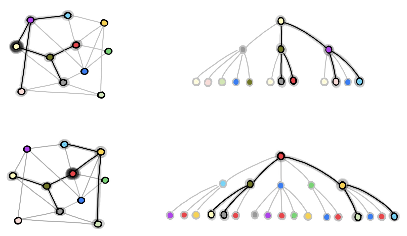
The first work to tackle the problem of scalability was GraphSAGE [8], a seminal paper of Will Hamilton and co-authors. GraphSAGE used neighbourhood sampling combined with mini-batch training to train GNNs on large graphs (the acronym SAGE, standing for “sample and aggregate”, is a reference to this scheme). The main idea is that in order to compute the training loss on a single node with an L-layer GCN, only the L-hop neighbours of that node are necessary, as nodes further away in the graph are not involved in the computation. The problem is that, for graphs of the “small-world” type, such as social networks, the 2-hop neighbourhood of some nodes may already contain millions of nodes, making it too big to be stored in memory [9]. GraphSAGE tackles this problem by sampling the neighbours up to the L-th hop: starting from the training node, it samples uniformly with replacement [10] a fixed number k of 1-hop neighbours, then for each of these neighbours it again samples k neighbours, and so on for L times. In this way, for every node we are guaranteed to have a bounded L-hop sampled neighbourhood of 𝒪(kᴸ) nodes. If we then construct a batch with b training nodes, each with its own independent L-hop neighbourhood, we get to a memory complexity of 𝒪(bkᴸ) independent of the graph size n. The computational complexity of one batch of GraphSAGE is 𝒪(bLd²kᴸ).

A notable drawback of GraphSAGE is that sampled nodes might appear multiple times, thus potentially introducing a lot of redundant computation. For instance, in the figure above the dark green node appears in both the l-hop neighbourhood for the two training nodes, and therefore its embedding is computed twice in the batch. With the increase of the batch size b and the number of samples k, the amount of redundant computation increases as well. Moreover, despite having 𝒪(bkᴸ) nodes in memory for each batch, the loss is computed on only b of them, and therefore, the computation for the other nodes is also in some sense wasted.
Multiple follow-up works focused on improving the sampling of mini-batches in order to remove redundant computation of GraphSAGE and make each batch more efficient. The most recent works in this direction are ClusterGCN [11] and GraphSAINT [12], which take the approach of graph-sampling (as opposed to neighbourhood-sampling of GraphSAGE). In graph-sampling approaches, for each batch, a subgraph of the original graph is sampled, and a full GCN-like model is run on the entire subgraph. The challenge is to make sure that these subgraphs preserve most of the original edges and still present a meaningful topological structure.
ClusterGCN achieves this by first clustering the graph. Then, at each batch, the model is trained on one cluster. This allows the nodes in each batch to be as tightly connected as possible.
GraphSAINTproposes instead a general probabilistic graph sampler constructing training batches by sampling subgraphs of the original graph. The graph sampler can be designed according to different schemes: for example, it can perform uniform node sampling, uniform edge sampling, or “importance sampling” by using random walks to compute the importance of nodes and use it as the probability distribution for sampling.
It is also important to note that one of the advantages of sampling is that during training it acts as a sort of edge-wise dropout, which regularises the model and can help the performance [13]. However, edge dropout would require to still see all the edges at inference time, which is not feasible here. Another effect graph sampling might have is reducing the bottleneck [14] and the resulting “over-squashing” phenomenon that stems from the exponential expansion of the neighbourhood.
Inour recent paper with Ben Chamberlain, Davide Eynard, and Federico Monti [15], we investigated the extent to which it is possible to design simple, sampling-free architectures for node-wise classification problems. You may wonder why one would prefer to abandon sampling strategies in light of the indirect benefits we have just highlighted above. There are a few reasons for that. First, instances of node classification problems may significantly vary from one another and, to the best of our knowledge, no work so far has systematically studied when sampling actually provides positive effects other than just alleviating computational complexity. Second, the implementation of sampling schemes introduces additional complexity and we believe a simple, strong, sampling-free, scalable baseline architecture is appealing.
Our approach is motivated by several recent empirical findings. First, simple fixed aggregators (such as GCN) were shown to often outperform in many cases more complex ones, such as GAT or MPNN [16]. Second, while deep learning success was built on models with a lot of layers, in graph deep learning it is still an open question whether depth is needed. In particular, Wu and coauthors [17] argue that a GCN model with a single multi-hop diffusion layer can perform on par with models with multiple layers.
By combining different, fixed neighbourhood aggregators within a single convolutional layer, it is possible to obtain an extremely scalable model without resorting to graph sampling [18]. In other words, all the graph related (fixed) operations are in the first layer of the architecture and can therefore be precomputed; the pre-aggregated information can then be fed as inputs to the rest of the model which, due to the lack of neighbourhood aggregation, boils down to a multi-layer perceptron (MLP). Importantly, the expressivity in the graph filtering operations can still be retained even with such a shallow convolutional scheme by employing several, possibly specialised and more complex, diffusion operators. As an example, it is possible to design operators to include local substructure counting [19] or graph motifs [20].
The proposed scalable architecture, which we call Scalable Inception-like Graph Network (SIGN) has the following form for node-wise classification tasks:
Y = softmax(ReLU(XW₀ | A₁XW₁ | A₂XW₂ | … | AᵣXWᵣ) W’)
Here Aᵣ are linear diffusion matrices (such as a normalised adjacency matrix, its powers, or a motif matrix) and Wᵣ and W’ are learnable parameters. As depicted in the figure above, the network can be made deeper with additional node-wise layers,
Y = softmax(ReLU(…ReLU(XW₀ | A₁XW₁ | … | AᵣXWᵣ) W’)… W’’)
Finally, when employing different powers for the same diffusion operator (e.g. A₁=B¹, A₂=B², etc.), the graph operations effectively aggregate from neighbours in further and further hops, akin to having convolutional filters of different receptive fields within the same network layer. This analogy to the popular inception module in classical CNNs explains the name of the proposed architecture [21].
As already mentioned, the matrix products A₁X,…, AᵣX in the above equations do not depend on the learnable model parameters and can thus be pre-computed. In particular, for very large graphs this pre-computation can be scaled efficiently using distributed computing infrastructures such as Apache Spark. This effectively reduces the computational complexity of the overall model to that of an MLP. Moreover, by moving the diffusion to the pre-computation step, we can aggregate information from all the neighbours, avoiding sampling and the possible loss of information and bias that comes with it [22].
The main advantage of SIGN is its scalability and efficiency, as it can be trained using standard mini-batch gradient descent. We found our model to be up to two orders of magnitude faster than ClusterGCN and GraphSAINT at inference time, while also being significantly faster at training time (all this while maintaining accuracy performances very close to that of the state-of-the-art GraphSAINT).

Moreover, our model supports any diffusion operators. For different types of graphs, different diffusion operators may be necessary, and we found some tasks to benefit from having motif-based operators such as triangle counts.
Despite the limitation of having only a single graph convolutional layer and linear diffusion operators, SIGN performs very well in practice, achieving results on par or even better than much more complex models. Given its speed and simplicity of implementation, we envision SIGN to be a simple baseline graph learning method for large-scale applications. Perhaps more importantly, the success of such a simple model leads to a more fundamental question: do we really need deep graph neural networks? We conjecture that in many problems of learning on social networks and “small world” graphs, we should use richer local structures rather than resort to brute-force deep architectures. Interestingly, traditional CNNs architectures evolved according to an opposite trend (deeper networks with smaller filters) because of computational advantages and the ability to compose complex features of simpler ones. We are not sure if the same approach is right for graphs, where compositionality is much more complex (e.g. certain structures cannot be computed by message passing, no matter how deep the network is). For sure, more elaborate experiments are still needed to test this conjecture.
[1] The recently introduced Open Graph Benchmark now offers large-scale graphs with millions of nodes. It will probably take some time for the community to switch to it.
[2] T. Kipf and M. Welling, Semi-supervised classification with graph convolutional networks (2017). Proc. ICLR introduced the popular GCN architecture, which was derived as a simplification of the ChebNet model proposed by M. Defferrard et al. Convolutional neural networks on graphs with fast localized spectral filtering (2016). Proc. NIPS.
[3] As the diffusion operator, Kipf and Welling used the graph adjacency matrix with self-loops (i.e., the node itself contributes to its feature update), but other choices are possible as well. The diffusion operation can be made feature-dependent of the form A(X)X (i.e., it is still a linear combination of the node features, but the weights depend on the features themselves) like in MoNet [4] or GAT [5] models, or completely nonlinear,𝒜(X), like in message-passing neural networks (MPNN) [6]. For simplicity, we focus the discussion on the GCN model applied to node-wise classification.
[4] F. Monti et al., Geometric Deep Learning on Graphs and Manifolds Using Mixture Model CNNs (2017). In Proc. CVPR.
[5] P. Veličković et al., Graph Attention Networks (2018). In Proc. ICLR.
[6] J. Gilmer et al., Neural message passing for quantum chemistry (2017). In Proc. ICML.
[7] Here we assume for simplicity that the graph is sparse with the number of edges |ℰ|=𝒪(n).
[8] W. Hamilton et al., Inductive Representation Learning on Large Graphs (2017). In Proc. NeurIPS.
[9] The number of neighbours in such graphs tends to grow exponentially with the neighbourhood expansion.
[10] Sampling with replacement means that some neighbour nodes can appear more than once, in particular if the number of neighbours is smaller than k.
[11] W.-L. Chiang et al., Cluster-GCN: An Efficient Algorithm for Training Deep and Large Graph Convolutional Networks (2019). In Proc. KDD.
[12] H. Zeng et al., GraphSAINT: Graph Sampling Based Inductive Learning Method (2020) In Proc. ICLR.
[13] Y. Rong et al. DropEdge: Towards deep graph convolutional networks on node classification (2020). In Proc. ICLR. An idea similar to DropOut where a random subset of edges is used during training.
[14] U. Alon and E. Yahav, On the bottleneck of graph neural networks and its practical implications (2020). arXiv:2006.05205. Identified the over-squashing phenomenon in graph neural networks, which is similar to one observed in sequential recurrent models.
[15] Frasca et al., SIGN: Scalable Inception Graph Neural Networks (2020). ICML workshop on Graph Representation Learning and Beyond.
[16] O. Shchur et al. Pitfalls of graph neural network evaluation (2018). Workshop on Relational Representation Learning. Shows that simple GNN models perform on par with more complex ones.
[17] F. Wu et al., Simplifying graph neural networks (2019). In Proc. ICML.
[18] While we stress that SIGN does not need sampling for computational efficiency, there are other reasons why graph subsampling is useful. J. Klicpera et al. Diffusion improves graph learning (2020). Proc. NeurIPS show that sampled diffusion matrices improve performance of graph neural networks. We observed the same phenomenon in early SIGN experiments.
[19] G. Bouritsas et al. Improving graph neural network expressivity via subgraph isomorphism counting (2020). arXiv:2006.09252. Shows how provably powerful GNNs can be obtained by structural node encoding.
[20] F. Monti, K. Otness, M. M. Bronstein, MotifNet: a motif-based graph convolutional network for directed graphs (2018). arXiv:1802.01572. Uses motif-based diffusion operators.
[21] C. Szegedi et al., Going deeper with convolution (2015). Proc. CVPR proposed the inception module in the already classical Google LeNet architecture. To be fair, we were not the first to think of graph inception modules. Our collaborator Anees Kazi from TU Munich, who was a visiting student at Imperial College last year, introduced them first.
[22] Note that reaching higher-order neighbours is normally achieved by depth-wise stacking graph convolutional layers operating with direct neighbours; in our architecture this is directly achieved in the first layer by powers of graph operators.


