Preprocessing, Model Design, Evaluation, Explainability for Bag-of-Words, Word Embedding, Language models
Summary
In this article, using NLP and Python, I will explain 3 different strategies for text multiclass classification: the old-fashioned Bag-of-Words (with Tf-Idf ), the famous Word Embedding (with Word2Vec), and the cutting edge Language models (with BERT).
NLP (Natural Language Processing) is the field of artificial intelligence that studies the interactions between computers and human languages, in particular how to program computers to process and analyze large amounts of natural language data. NLP is often applied for classifying text data. Text classification is the problem of assigning categories to text data according to its content.
There are different techniques to extract information from raw text data and use it to train a classification model. This tutorial compares the old school approach of Bag-of-Words (used with a simple machine learning algorithm), the popular Word Embedding model (used with a deep learning neural network), and the state of the art Language models (used with transfer learning from attention-based transformers) that have completely revolutionized the NLP landscape.
I will present some useful Python code that can be easily applied in other similar cases (just copy, paste, run) and walk through every line of code with comments so that you can replicate this example (link to the full code below).mdipietro09/DataScience_ArtificialIntelligence_UtilsPermalink Dismiss GitHub is home to over 50 million developers working together to host and review code, manage…github.com
I will use the “News category dataset” in which you are provided with news headlines from the year 2012 to 2018 obtained from HuffPost and you are asked to classify them with the right category, therefore this is a multiclass classification problem (link below).News Category DatasetIdentify the type of news based on headlines and short descriptionswww.kaggle.com
In particular, I will go through:
- Setup: import packages, read data, Preprocessing, Partitioning.
- Bag-of-Words: Feature Engineering & Feature Selection & Machine Learning with scikit-learn, Testing & Evaluation, Explainability with lime.
- Word Embedding: Fitting a Word2Vec with gensim, Feature Engineering & Deep Learning with tensorflow/keras, Testing & Evaluation, Explainability with the Attention mechanism.
- Language Models: Feature Engineering with transformers, Transfer Learning from pre-trained BERT with transformers and tensorflow/keras, Testing & Evaluation.
Setup
First of all, I need to import the following libraries:
## for data
import json
import pandas as pd
import numpy as np## for plotting
import matplotlib.pyplot as plt
import seaborn as sns## for processing
import re
import nltk## for bag-of-words
from sklearn import feature_extraction, model_selection, naive_bayes, pipeline, manifold, preprocessing## for explainer
from lime import lime_text## for word embedding
import gensim
import gensim.downloader as gensim_api## for deep learning
from tensorflow.keras import models, layers, preprocessing as kprocessing
from tensorflow.keras import backend as K## for bert language model
import transformers
The dataset is contained into a json file, so I will first read it into a list of dictionaries with json and then transform it into a pandas Dataframe.
lst_dics = []
with open('data.json', mode='r', errors='ignore') as json_file:
    for dic in json_file:
        lst_dics.append( json.loads(dic) )## print the first one
lst_dics[0]

The original dataset contains over 30 categories, but for the purposes of this tutorial, I will work with a subset of 3: Entertainment, Politics, and Tech.
## create dtf
dtf = pd.DataFrame(lst_dics)## filter categories
dtf = dtf[ dtf["category"].isin(['ENTERTAINMENT','POLITICS','TECH']) ][["category","headline"]]## rename columns
dtf = dtf.rename(columns={"category":"y", "headline":"text"})## print 5 random rows
dtf.sample(5)
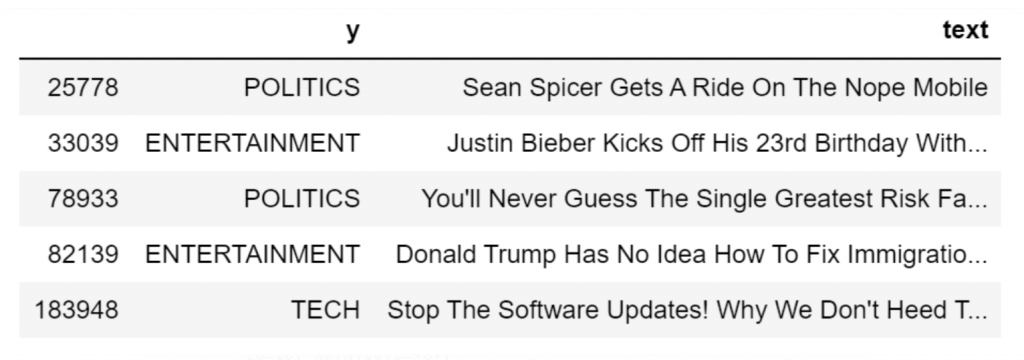
In order to understand the composition of the dataset, I am going to look into the univariate distribution of the target by showing labels frequency with a bar plot.
fig, ax = plt.subplots()
fig.suptitle("y", fontsize=12)
dtf["y"].reset_index().groupby("y").count().sort_values(by=
       "index").plot(kind="barh", legend=False,
        ax=ax).grid(axis='x')
plt.show()
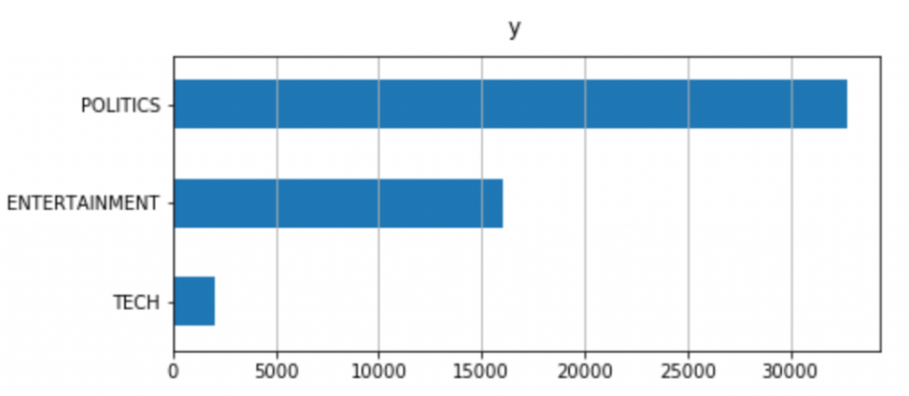
The dataset is imbalanced: the proportion of Tech news is really small compared to the others, this will make for models to recognize Tech news rather tough.
Before explaining and building the models, I am going to give an example of preprocessing by cleaning text, removing stop words, and applying lemmatization. I will write a function and apply it to the whole data set.
'''
Preprocess a string.
:parameter
    :param text: string - name of column containing text
    :param lst_stopwords: list - list of stopwords to remove
    :param flg_stemm: bool - whether stemming is to be applied
    :param flg_lemm: bool - whether lemmitisation is to be applied
:return
    cleaned text
'''
def utils_preprocess_text(text, flg_stemm=False, flg_lemm=True, lst_stopwords=None):
    ## clean (convert to lowercase and remove punctuations and
    characters and then strip)
    text = re.sub(r'[^\w\s]', '', str(text).lower().strip())

    ## Tokenize (convert from string to list)
    lst_text = text.split()    ## remove Stopwords
    if lst_stopwords is not None:
        lst_text = [word for word in lst_text if word not in
                    lst_stopwords]

    ## Stemming (remove -ing, -ly, ...)
    if flg_stemm == True:
        ps = nltk.stem.porter.PorterStemmer()
        lst_text = [ps.stem(word) for word in lst_text]

    ## Lemmatisation (convert the word into root word)
    if flg_lemm == True:
        lem = nltk.stem.wordnet.WordNetLemmatizer()
        lst_text = [lem.lemmatize(word) for word in lst_text]

    ## back to string from list
    text = " ".join(lst_text)
    return text
That function removes a set of words from the corpus if given. I can create a list of generic stop words for the English vocabulary with nltk (we could edit this list by adding or removing words).
lst_stopwords = nltk.corpus.stopwords.words("english")
lst_stopwords

Now I shall apply the function I wrote on the whole dataset and store the result in a new column named “text_clean” so that you can choose to work with the raw corpus or the preprocessed text.
dtf["text_clean"] = dtf["text"].apply(lambda x:
          utils_preprocess_text(x, flg_stemm=False, flg_lemm=True,
          lst_stopwords=lst_stopwords))dtf.head()

If you are interested in a deeper text analysis and preprocessing, you can check this article. With this in mind, I am going to partition the dataset into training set (70%) and test set (30%) in order to evaluate the models performance.
## split dataset
dtf_train, dtf_test = model_selection.train_test_split(dtf, test_size=0.3)## get target
y_train = dtf_train["y"].values
y_test = dtf_test["y"].values
Let’s get started, shall we?
Bag-of-Words
The Bag-of-Words model is simple: it builds a vocabulary from a corpus of documents and counts how many times the words appear in each document. To put it another way, each word in the vocabulary becomes a feature and a document is represented by a vector with the same length of the vocabulary (a “bag of words”). For instance, let’s take 3 sentences and represent them with this approach:

As you can imagine, this approach causes a significant dimensionality problem: the more documents you have the larger is the vocabulary, so the feature matrix will be a huge sparse matrix. Therefore, the Bag-of-Words model is usually preceded by an important preprocessing (word cleaning, stop words removal, stemming/lemmatization) aimed to reduce the dimensionality problem.
Terms frequency is not necessarily the best representation for text. In fact, you can find in the corpus common words with the highest frequency but little predictive power over the target variable. To address this problem there is an advanced variant of the Bag-of-Words that, instead of simple counting, uses the term frequency–inverse document frequency (or Tf–Idf). Basically, the value of a word increases proportionally to count, but it is inversely proportional to the frequency of the word in the corpus.
Let’s start with the Feature Engineering, the process to create features by extracting information from the data. I am going to use the Tf-Idf vectorizer with a limit of 10,000 words (so the length of my vocabulary will be 10k), capturing unigrams (i.e. “new” and “york”) and bigrams (i.e. “new york”). I will provide the code for the classic count vectorizer as well:
## Count (classic BoW)
vectorizer = feature_extraction.text.CountVectorizer(max_features=10000, ngram_range=(1,2))

## Tf-Idf (advanced variant of BoW)
vectorizer = feature_extraction.text.TfidfVectorizer(max_features=10000, ngram_range=(1,2))
Now I will use the vectorizer on the preprocessed corpus of the train set to extract a vocabulary and create the feature matrix.
corpus = dtf_train["text_clean"]vectorizer.fit(corpus)
X_train = vectorizer.transform(corpus)
dic_vocabulary = vectorizer.vocabulary_
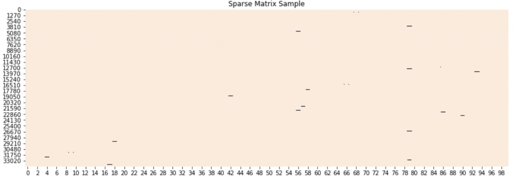
The feature matrix X_train has a shape of 34,265 (Number of documents in training) x 10,000 (Length of vocabulary) and it’s pretty sparse:
sns.heatmap(X_train.todense()[:,np.random.randint(0,X.shape[1],100)]==0, vmin=0, vmax=1, cbar=False).set_title('Sparse Matrix Sample')
In order to know the position of a certain word, we can look it up in the vocabulary:
word = "new york"dic_vocabulary[word]
If the word exists in the vocabulary, this command prints a number N, meaning that the Nth feature of the matrix is that word.
In order to drop some columns and reduce the matrix dimensionality, we can carry out some Feature Selection, the process of selecting a subset of relevant variables. I will proceed as follows:
- treat each category as binary (for example, the “Tech” category is 1 for the Tech news and 0 for the others);
- perform a Chi-Square test to determine whether a feature and the (binary) target are independent;
- keep only the features with a certain p-value from the Chi-Square test.
y = dtf_train["y"]
X_names = vectorizer.get_feature_names()
p_value_limit = 0.95dtf_features = pd.DataFrame()
for cat in np.unique(y):
    chi2, p = feature_selection.chi2(X_train, y==cat)
    dtf_features = dtf_features.append(pd.DataFrame(
                   {"feature":X_names, "score":1-p, "y":cat}))
    dtf_features = dtf_features.sort_values(["y","score"],
                    ascending=[True,False])
    dtf_features = dtf_features[dtf_features["score"]>p_value_limit]X_names = dtf_features["feature"].unique().tolist()
I reduced the number of features from 10,000 to 3,152 by keeping the most statistically relevant ones. Let’s print some:
for cat in np.unique(y):
   print("# {}:".format(cat))
   print("  . selected features:",
         len(dtf_features[dtf_features["y"]==cat]))
   print("  . top features:", ",".join(
dtf_features[dtf_features["y"]==cat]["feature"].values[:10]))
   print(" ")

We can refit the vectorizer on the corpus by giving this new set of words as input. That will produce a smaller feature matrix and a shorter vocabulary.
vectorizer = feature_extraction.text.TfidfVectorizer(vocabulary=X_names)vectorizer.fit(corpus)
X_train = vectorizer.transform(corpus)
dic_vocabulary = vectorizer.vocabulary_
The new feature matrix X_train has a shape of is 34,265 (Number of documents in training) x 3,152 (Length of the given vocabulary). Let’s see if the matrix is less sparse:
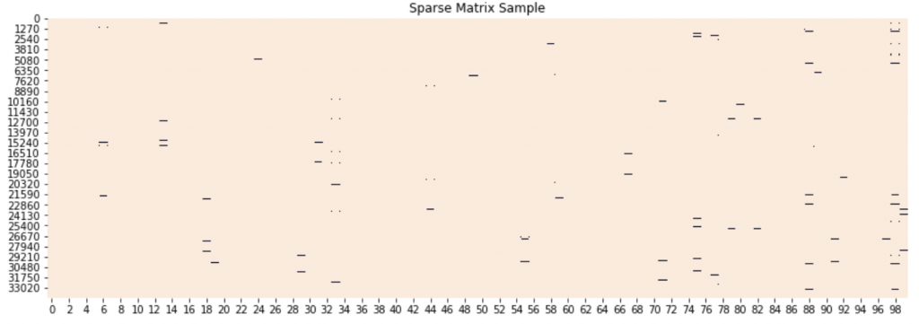
It’s time to train a machine learning model and test it. I recommend using a Naive Bayes algorithm: a probabilistic classifier that makes use of Bayes’ Theorem, a rule that uses probability to make predictions based on prior knowledge of conditions that might be related. This algorithm is the most suitable for such large dataset as it considers each feature independently, calculates the probability of each category, and then predicts the category with the highest probability.
classifier = naive_bayes.MultinomialNB()
I’m going to train this classifier on the feature matrix and then test it on the transformed test set. To that end, I need to build a scikit-learn pipeline: a sequential application of a list of transformations and a final estimator. Putting the Tf-Idf vectorizer and the Naive Bayes classifier in a pipeline allows us to transform and predict test data in just one step.
## pipeline
model = pipeline.Pipeline([("vectorizer", vectorizer),
                           ("classifier", classifier)])## train classifier
model["classifier"].fit(X_train, y_train)## test
X_test = dtf_test["text_clean"].values
predicted = model.predict(X_test)
predicted_prob = model.predict_proba(X_test)
We can now evaluate the performance of the Bag-of-Words model, I will use the following metrics:
- Accuracy: the fraction of predictions the model got right.
- Confusion Matrix: a summary table that breaks down the number of correct and incorrect predictions by each class.
- ROC: a plot that illustrates the true positive rate against the false positive rate at various threshold settings. The area under the curve (AUC) indicates the probability that the classifier will rank a randomly chosen positive observation higher than a randomly chosen negative one.
- Precision: the fraction of relevant instances among the retrieved instances.
- Recall: the fraction of the total amount of relevant instances that were actually retrieved.
classes = np.unique(y_test)
y_test_array = pd.get_dummies(y_test, drop_first=False).values
    ## Accuracy, Precision, Recall
accuracy = metrics.accuracy_score(y_test, predicted)
auc = metrics.roc_auc_score(y_test, predicted_prob,
                            multi_class="ovr")
print("Accuracy:",  round(accuracy,2))
print("Auc:", round(auc,2))
print("Detail:")
print(metrics.classification_report(y_test, predicted))

## Plot confusion matrix
cm = metrics.confusion_matrix(y_test, predicted)
fig, ax = plt.subplots()
sns.heatmap(cm, annot=True, fmt='d', ax=ax, cmap=plt.cm.Blues,
            cbar=False)
ax.set(xlabel="Pred", ylabel="True", xticklabels=classes,
       yticklabels=classes, title="Confusion matrix")
plt.yticks(rotation=0)
fig, ax = plt.subplots(nrows=1, ncols=2)
## Plot roc
for i in range(len(classes)):
    fpr, tpr, thresholds = metrics.roc_curve(y_test_array[:,i],
                           predicted_prob[:,i])
    ax[0].plot(fpr, tpr, lw=3,
              label='{0} (area={1:0.2f})'.format(classes[i],
                              metrics.auc(fpr, tpr))
               )
ax[0].plot([0,1], [0,1], color='navy', lw=3, linestyle='--')
ax[0].set(xlim=[-0.05,1.0], ylim=[0.0,1.05],
          xlabel='False Positive Rate',
          ylabel="True Positive Rate (Recall)",
          title="Receiver operating characteristic")
ax[0].legend(loc="lower right")
ax[0].grid(True)

## Plot precision-recall curve
for i in range(len(classes)):
    precision, recall, thresholds = metrics.precision_recall_curve(
                 y_test_array[:,i], predicted_prob[:,i])
    ax[1].plot(recall, precision, lw=3,
               label='{0} (area={1:0.2f})'.format(classes[i],
                                  metrics.auc(recall, precision))
              )
ax[1].set(xlim=[0.0,1.05], ylim=[0.0,1.05], xlabel='Recall',
          ylabel="Precision", title="Precision-Recall curve")
ax[1].legend(loc="best")
ax[1].grid(True)
plt.show()
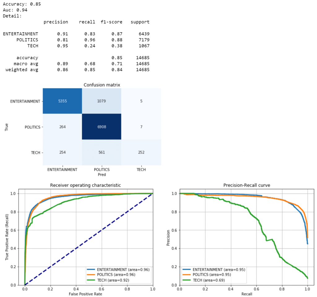
The BoW model got 85% of the test set right (Accuracy is 0.85), but struggles to recognize Tech news (only 252 predicted correctly).
Let’s try to understand why the model classifies news with a certain category and assess the explainability of these predictions. The lime package can help us to build an explainer. To give an illustration, I will take a random observation from the test set and see what the model predicts and why.
## select observation
i = 0
txt_instance = dtf_test["text"].iloc[i]## check true value and predicted value
print("True:", y_test[i], "--> Pred:", predicted[i], "| Prob:", round(np.max(predicted_prob[i]),2))## show explanation
explainer = lime_text.LimeTextExplainer(class_names=
             np.unique(y_train))
explained = explainer.explain_instance(txt_instance,
             model.predict_proba, num_features=3)
explained.show_in_notebook(text=txt_instance, predict_proba=False)

That makes sense: the words “Clinton” and “GOP” pointed the model in the right direction (Politics news) even if the word “Stage” is more common among Entertainment news.
Word Embedding
Word Embedding is the collective name for feature learning techniques where words from the vocabulary are mapped to vectors of real numbers. These vectors are calculated from the probability distribution for each word appearing before or after another. To put it another way, words of the same context usually appear together in the corpus, so they will be close in the vector space as well. For instance, let’s take the 3 sentences from the previous example:
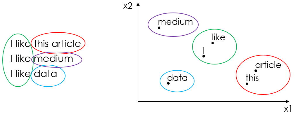
In this tutorial, I’m going to use the first model of this family: Google’s Word2Vec (2013). Other popular Word Embedding models are Stanford’s GloVe (2014)and Facebook’s FastText (2016).
Word2Vec produces a vector space, typically of several hundred dimensions, with each unique word in the corpus such that words that share common contexts in the corpus are located close to one another in the space. That can be done using 2 different approaches: starting from a single word to predict its context (Skip-gram) or starting from the context to predict a word (Continuous Bag-of-Words).
In Python, you can load a pre-trained Word Embedding model from genism-data like this:
nlp = gensim_api.load("word2vec-google-news-300")
Instead of using a pre-trained model, I am going to fit my own Word2Vec on the training data corpus with gensim. Before fitting the model, the corpus needs to be transformed into a list of lists of n-grams. In this particular case, I’ll try to capture unigrams (“york”), bigrams (“new york”), and trigrams (“new york city”).
corpus = dtf_train["text_clean"]
## create list of lists of unigrams
lst_corpus = []
for string in corpus:
   lst_words = string.split()
   lst_grams = [" ".join(lst_words[i:i+1])
               for i in range(0, len(lst_words), 1)]
   lst_corpus.append(lst_grams)
## detect bigrams and trigrams
bigrams_detector = gensim.models.phrases.Phrases(lst_corpus,
                 delimiter=" ".encode(), min_count=5, threshold=10)
bigrams_detector = gensim.models.phrases.Phraser(bigrams_detector)trigrams_detector = gensim.models.phrases.Phrases(bigrams_detector[lst_corpus],
            delimiter=" ".encode(), min_count=5, threshold=10)
trigrams_detector = gensim.models.phrases.Phraser(trigrams_detector)
When fitting the Word2Vec, you need to specify:
- the target size of the word vectors, I’ll use 300;
- the window, or the maximum distance between the current and predicted word within a sentence, I’ll use the mean length of text in the corpus;
- the training algorithm, I’ll use skip-grams (sg=1) as in general it has better results.
## fit w2v
nlp = gensim.models.word2vec.Word2Vec(lst_corpus, size=300,
            window=8, min_count=1, sg=1, iter=30)
We have our embedding model, so we can select any word from the corpus and transform it into a vector.
word = "data"
nlp[word].shape
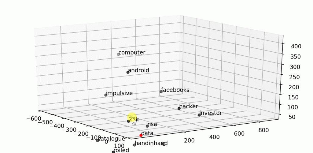
We can even use it to visualize a word and its context into a smaller dimensional space (2D or 3D) by applying any dimensionality reduction algorithm (i.e. TSNE).
word = "data"
fig = plt.figure()## word embedding
tot_words = [word] + [tupla[0] for tupla in
                 nlp.most_similar(word, topn=20)]
X = nlp[tot_words]## pca to reduce dimensionality from 300 to 3
pca = manifold.TSNE(perplexity=40, n_components=3, init='pca')
X = pca.fit_transform(X)## create dtf
dtf_ = pd.DataFrame(X, index=tot_words, columns=["x","y","z"])
dtf_["input"] = 0
dtf_["input"].iloc[0:1] = 1## plot 3d
from mpl_toolkits.mplot3d import Axes3D
ax = fig.add_subplot(111, projection='3d')
ax.scatter(dtf_[dtf_["input"]==0]['x'],
           dtf_[dtf_["input"]==0]['y'],
           dtf_[dtf_["input"]==0]['z'], c="black")
ax.scatter(dtf_[dtf_["input"]==1]['x'],
           dtf_[dtf_["input"]==1]['y'],
           dtf_[dtf_["input"]==1]['z'], c="red")
ax.set(xlabel=None, ylabel=None, zlabel=None, xticklabels=[],
       yticklabels=[], zticklabels=[])
for label, row in dtf_[["x","y","z"]].iterrows():
    x, y, z = row
    ax.text(x, y, z, s=label)

That’s pretty cool and all, but how can the word embedding be useful to predict the news category? Well, the word vectors can be used in a neural network as weights. This is how:
- First, transform the corpus into padded sequences of word ids to get a feature matrix.
- Then, create an embedding matrix so that the vector of the word with id N is located at the Nth row.
- Finally, build a neural network with an embedding layer that weighs every word in the sequences with the corresponding vector.
Let’s start with the Feature Engineering by transforming the same preprocessed corpus (list of lists of n-grams) given to the Word2Vec into a list of sequences using tensorflow/keras:
## tokenize text
tokenizer = kprocessing.text.Tokenizer(lower=True, split=' ',
                     oov_token="NaN",
                     filters='!"#$%&()*+,-./:;<=>?@[\\]^_`{|}~\t\n')
tokenizer.fit_on_texts(lst_corpus)
dic_vocabulary = tokenizer.word_index## create sequence
lst_text2seq= tokenizer.texts_to_sequences(lst_corpus)## padding sequence
X_train = kprocessing.sequence.pad_sequences(lst_text2seq,
                    maxlen=15, padding="post", truncating="post")
The feature matrix X_train has a shape of 34,265 x 15 (Number of sequences x Sequences max length). Let’s visualize it:
sns.heatmap(X_train==0, vmin=0, vmax=1, cbar=False)
plt.show()

Every text in the corpus is now an id sequence with length 15. For instance, if a text had 10 tokens in it, then the sequence is composed of 10 ids + 5 0s, which is the padding element (while the id for word not in the vocabulary is 1). Let’s print how a text from the train set has been transformed into a sequence with the padding and the vocabulary.
i = 0

## list of text: ["I like this", ...]
len_txt = len(dtf_train["text_clean"].iloc[i].split())
print("from: ", dtf_train["text_clean"].iloc[i], "| len:", len_txt)

## sequence of token ids: [[1, 2, 3], ...]
len_tokens = len(X_train[i])
print("to: ", X_train[i], "| len:", len(X_train[i]))

## vocabulary: {"I":1, "like":2, "this":3, ...}
print("check: ", dtf_train["text_clean"].iloc[i].split()[0],
      " -- idx in vocabulary -->",
      dic_vocabulary[dtf_train["text_clean"].iloc[i].split()[0]])

print("vocabulary: ", dict(list(dic_vocabulary.items())[0:5]), "... (padding element, 0)")

Before moving on, don’t forget to do the same feature engineering on the test set as well:
corpus = dtf_test["text_clean"]
## create list of n-grams
lst_corpus = []
for string in corpus:
    lst_words = string.split()
    lst_grams = [" ".join(lst_words[i:i+1]) for i in range(0,
                 len(lst_words), 1)]
    lst_corpus.append(lst_grams)
    ## detect common bigrams and trigrams using the fitted detectors
lst_corpus = list(bigrams_detector[lst_corpus])
lst_corpus = list(trigrams_detector[lst_corpus])
## text to sequence with the fitted tokenizer
lst_text2seq = tokenizer.texts_to_sequences(lst_corpus)
## padding sequence
X_test = kprocessing.sequence.pad_sequences(lst_text2seq, maxlen=15,
             padding="post", truncating="post")

We’ve got our X_train and X_test, now we need to create the matrix of embedding that will be used as a weight matrix in the neural network classifier.
## start the matrix (length of vocabulary x vector size) with all 0s
embeddings = np.zeros((len(dic_vocabulary)+1, 300))for word,idx in dic_vocabulary.items():
    ## update the row with vector
    try:
        embeddings[idx] =  nlp[word]
    ## if word not in model then skip and the row stays all 0s
    except:
        pass
That code generates a matrix of shape 22,338 x 300 (Length of vocabulary extracted from the corpus x Vector size). It can be navigated by word id, which can be obtained from the vocabulary.
word = "data"print("dic[word]:", dic_vocabulary[word], "|idx")
print("embeddings[idx]:", embeddings[dic_vocabulary[word]].shape,
      "|vector")

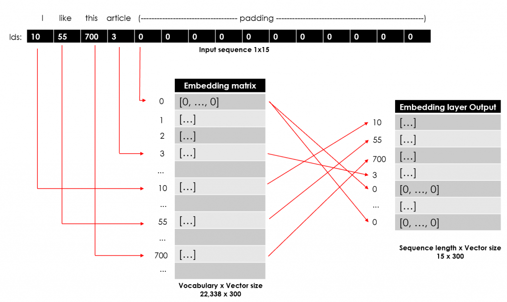
It’s finally time to build a deep learning model. I’m going to use the embedding matrix in the first Embedding layer of the neural network that I will build and train to classify the news. Each id in the input sequence will be used as the index to access the embedding matrix. The output of this Embedding layer will be a 2D matrix with a word vector for each word id in the input sequence (Sequence length x Vector size). Let’s use the sentence “I like this article” as an example:
My neural network shall be structured as follows:
- an Embedding layer that takes the sequences as input and the word vectors as weights, just as described before.
- A simple Attention layer that won’t affect the predictions but it’s going to capture the weights of each instance and allow us to build a nice explainer (it isn’t necessary for the predictions, just for the explainability, so you can skip it). The Attention mechanism was presented in this paper (2014) as a solution to the problem of the sequence models (i.e. LSTM) to understand what parts of a long text are actually relevant.
- Two layers of Bidirectional LSTM to model the order of words in a sequence in both directions.
- Two final dense layers that will predict the probability of each news category.
## code attention layer
def attention_layer(inputs, neurons):
    x = layers.Permute((2,1))(inputs)
    x = layers.Dense(neurons, activation="softmax")(x)
    x = layers.Permute((2,1), name="attention")(x)
    x = layers.multiply([inputs, x])
    return x
## input
x_in = layers.Input(shape=(15,))## embedding
x = layers.Embedding(input_dim=embeddings.shape[0],
                     output_dim=embeddings.shape[1],
                     weights=[embeddings],
                     input_length=15, trainable=False)(x_in)## apply attention
x = attention_layer(x, neurons=15)## 2 layers of bidirectional lstm
x = layers.Bidirectional(layers.LSTM(units=15, dropout=0.2,
                         return_sequences=True))(x)
x = layers.Bidirectional(layers.LSTM(units=15, dropout=0.2))(x)## final dense layers
x = layers.Dense(64, activation='relu')(x)
y_out = layers.Dense(3, activation='softmax')(x)## compile
model = models.Model(x_in, y_out)
model.compile(loss='sparse_categorical_crossentropy',
              optimizer='adam', metrics=['accuracy'])

model.summary()
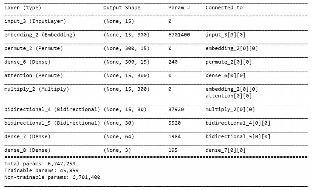
Now we can train the model and check the performance on a subset of the training set used for validation before testing it on the actual test set.
## encode y
dic_y_mapping = {n:label for n,label in
                 enumerate(np.unique(y_train))}
inverse_dic = {v:k for k,v in dic_y_mapping.items()}
y_train = np.array([inverse_dic[y] for y in y_train])## train
training = model.fit(x=X_train, y=y_train, batch_size=256,
                     epochs=10, shuffle=True, verbose=0,
                     validation_split=0.3)## plot loss and accuracy
metrics = [k for k in training.history.keys() if ("loss" not in k) and ("val" not in k)]
fig, ax = plt.subplots(nrows=1, ncols=2, sharey=True)ax[0].set(title="Training")
ax11 = ax[0].twinx()
ax[0].plot(training.history['loss'], color='black')
ax[0].set_xlabel('Epochs')
ax[0].set_ylabel('Loss', color='black')
for metric in metrics:
    ax11.plot(training.history[metric], label=metric)
ax11.set_ylabel("Score", color='steelblue')
ax11.legend()ax[1].set(title="Validation")
ax22 = ax[1].twinx()
ax[1].plot(training.history['val_loss'], color='black')
ax[1].set_xlabel('Epochs')
ax[1].set_ylabel('Loss', color='black')
for metric in metrics:
     ax22.plot(training.history['val_'+metric], label=metric)
ax22.set_ylabel("Score", color="steelblue")
plt.show()

Nice! In some epochs, the accuracy reached 0.89. In order to complete the evaluation of the Word Embedding model, let’s predict the test set and compare the same metrics used before (code for metrics is the same as before).
## test
predicted_prob = model.predict(X_test)
predicted = [dic_y_mapping[np.argmax(pred)] for pred in
             predicted_prob]
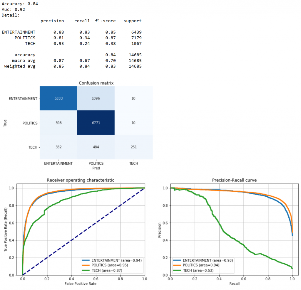
The model performs as good as the previous one, in fact, it also struggles to classify Tech news.
But is it explainable as well? Yes, it is! I put an Attention layer in the neural network to extract the weights of each word and understand how much those contributed to classify an instance. So I’ll try to use Attention weights to build an explainer (similar to the one seen in the previous section):
## select observation
i = 0
txt_instance = dtf_test["text"].iloc[i]## check true value and predicted value
print("True:", y_test[i], "--> Pred:", predicted[i], "| Prob:", round(np.max(predicted_prob[i]),2))
## show explanation
### 1. preprocess input
lst_corpus = []
for string in [re.sub(r'[^\w\s]','', txt_instance.lower().strip())]:
    lst_words = string.split()
    lst_grams = [" ".join(lst_words[i:i+1]) for i in range(0,
                 len(lst_words), 1)]
    lst_corpus.append(lst_grams)
lst_corpus = list(bigrams_detector[lst_corpus])
lst_corpus = list(trigrams_detector[lst_corpus])
X_instance = kprocessing.sequence.pad_sequences(
              tokenizer.texts_to_sequences(corpus), maxlen=15,
              padding="post", truncating="post")### 2. get attention weights
layer = [layer for layer in model.layers if "attention" in
         layer.name][0]
func = K.function([model.input], [layer.output])
weights = func(X_instance)[0]
weights = np.mean(weights, axis=2).flatten()### 3. rescale weights, remove null vector, map word-weight
weights = preprocessing.MinMaxScaler(feature_range=(0,1)).fit_transform(np.array(weights).reshape(-1,1)).reshape(-1)
weights = [weights[n] for n,idx in enumerate(X_instance[0]) if idx
           != 0]
dic_word_weigth = {word:weights[n] for n,word in
                   enumerate(lst_corpus[0]) if word in
                   tokenizer.word_index.keys()}### 4. barplot
if len(dic_word_weigth) > 0:
   dtf = pd.DataFrame.from_dict(dic_word_weigth, orient='index',
                                columns=["score"])
   dtf.sort_values(by="score",
           ascending=True).tail(top).plot(kind="barh",
           legend=False).grid(axis='x')
   plt.show()
else:
   print("--- No word recognized ---")### 5. produce html visualization
text = []
for word in lst_corpus[0]:
    weight = dic_word_weigth.get(word)
    if weight is not None:
         text.append('<b><span style="background-color:rgba(100,149,237,' + str(weight) + ');">' + word + '</span></b>')
    else:
         text.append(word)
text = ' '.join(text)### 6. visualize on notebook
print("\033[1m"+"Text with highlighted words")
from IPython.core.display import display, HTML
display(HTML(text))
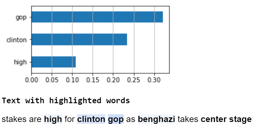
Just like before, the words “clinton” and “gop” activated the neurons of the model, but this time also “high” and “benghazi” have been considered slightly relevant for the prediction.
Language Models
Language Models, or Contextualized/Dynamic Word Embeddings, overcome the biggest limitation of the classic Word Embedding approach: polysemy disambiguation, a word with different meanings (e.g. “ bank” or “stick”) is identified by just one vector. One of the first popular ones was ELMO (2018), which doesn’t apply a fixed embedding but, using a bidirectional LSTM, looks at the entire sentence and then assigns an embedding to each word.
Enter Transformers: a new modeling technique presented by Google’s paper Attention is All You Need(2017)in which it was demonstrated that sequence models (like LSTM) can be totally replaced by Attention mechanisms, even obtaining better performances.
Google’s BERT(Bidirectional Encoder Representations from Transformers, 2018) combines ELMO context embedding and several Transformers, plus it’s bidirectional (which was a big novelty for Transformers). The vector BERT assigns to a word is a function of the entire sentence, therefore, a word can have different vectors based on the contexts. Let’s try it using transformers:
txt = "bank river"## bert tokenizer
tokenizer = transformers.BertTokenizer.from_pretrained('bert-base-uncased', do_lower_case=True)## bert model
nlp = transformers.TFBertModel.from_pretrained('bert-base-uncased')## return hidden layer with embeddings
input_ids = np.array(tokenizer.encode(txt))[None,:]
embedding = nlp(input_ids)embedding[0][0]

If we change the input text into “bank money”, we get this instead:

In order to complete a text classification task, you can use BERT in 3 different ways:
- train it all from scratches and use it as classifier.
- Extract the word embeddings and use them in an embedding layer (like I did with Word2Vec).
- Fine-tuning the pre-trained model (transfer learning).
I’m going with the latter and do transfer learning from a pre-trained lighter version of BERT, called Distil-BERT (66 million of parameters instead of 110 million!).
## distil-bert tokenizer
tokenizer = transformers.AutoTokenizer.from_pretrained('distilbert-base-uncased', do_lower_case=True)
As usual, before fitting the model there is some Feature Engineering to do, but this time it’s gonna be a little trickier. To give an illustration of what I’m going to do, let’s take as an example our beloved sentence “I like this article”, which has to be transformed into 3 vectors (Ids, Mask, Segment):

First of all, we need to select the sequence max length. This time I’m gonna choose a much larger number (i.e. 50) because BERT splits unknown words into sub-tokens until it finds a known unigrams. For example, if a made-up word like “zzdata” is given, BERT would split it into [“z”, “##z”, “##data”]. Moreover, we have to insert special tokens into the input text, then generate masks and segments. Finally, put all together in a tensor to get the feature matrix that will have the shape of 3 (ids, masks, segments) x Number of documents in the corpus x Sequence length.
Please note that I’m using the raw text as corpus (so far I’ve been using the clean_text column).
corpus = dtf_train["text"]
maxlen = 50
## add special tokens
maxqnans = np.int((maxlen-20)/2)
corpus_tokenized = ["[CLS] "+
             " ".join(tokenizer.tokenize(re.sub(r'[^\w\s]+|\n', '',
             str(txt).lower().strip()))[:maxqnans])+
             " [SEP] " for txt in corpus]

## generate masks
masks = [[1]*len(txt.split(" ")) + [0]*(maxlen - len(
           txt.split(" "))) for txt in corpus_tokenized]

## padding
txt2seq = [txt + " [PAD]"*(maxlen-len(txt.split(" "))) if len(txt.split(" ")) != maxlen else txt for txt in corpus_tokenized]

## generate idx
idx = [tokenizer.encode(seq.split(" ")) for seq in txt2seq]

## generate segments
segments = []
for seq in txt2seq:
    temp, i = [], 0
    for token in seq.split(" "):
        temp.append(i)
        if token == "[SEP]":
             i += 1
    segments.append(temp)## feature matrix
X_train = [np.asarray(idx, dtype='int32'),
           np.asarray(masks, dtype='int32'),
           np.asarray(segments, dtype='int32')]
The feature matrix X_train has a shape of 3 x 34,265 x 50. We can check a random observation from the feature matrix:
i = 0print("txt: ", dtf_train["text"].iloc[0])
print("tokenized:", [tokenizer.convert_ids_to_tokens(idx) for idx in X_train[0][i].tolist()])
print("idx: ", X_train[0][i])
print("mask: ", X_train[1][i])
print("segment: ", X_train[2][i])
![take the same code and apply it to dtf_test[“text”] to get X_test.](https://resources.experfy.com/wp-content/uploads/2021/05/1vRUkclqzuGDvmgu1VFs-5A-1024x262.png)
You can take the same code and apply it to dtf_test[“text”] to get X_test.
Now, I’m going to build the deep learning model with transfer learning from the pre-trained BERT. Basically, I’m going to summarize the output of BERT into one vector with Average Pooling and then add two final Dense layers to predict the probability of each news category.
If you want to use the original versions of BERT, here’s the code (remember to redo the feature engineering with the right tokenizer):
## inputs
idx = layers.Input((50), dtype="int32", name="input_idx")
masks = layers.Input((50), dtype="int32", name="input_masks")
segments = layers.Input((50), dtype="int32", name="input_segments")## pre-trained bert
nlp = transformers.TFBertModel.from_pretrained("bert-base-uncased")
bert_out, _ = nlp([idx, masks, segments])## fine-tuning
x = layers.GlobalAveragePooling1D()(bert_out)
x = layers.Dense(64, activation="relu")(x)
y_out = layers.Dense(len(np.unique(y_train)),
                     activation='softmax')(x)## compile
model = models.Model([idx, masks, segments], y_out)for layer in model.layers[:4]:
    layer.trainable = Falsemodel.compile(loss='sparse_categorical_crossentropy',
              optimizer='adam', metrics=['accuracy'])model.summary()
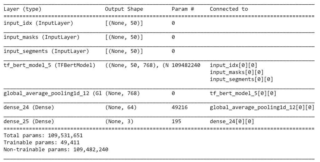
As I said, I’m going to use the lighter version instead, Distil-BERT:
## inputs
idx = layers.Input((50), dtype="int32", name="input_idx")
masks = layers.Input((50), dtype="int32", name="input_masks")## pre-trained bert with config
config = transformers.DistilBertConfig(dropout=0.2,
           attention_dropout=0.2)
config.output_hidden_states = Falsenlp = transformers.TFDistilBertModel.from_pretrained('distilbert-
                  base-uncased', config=config)
bert_out = nlp(idx, attention_mask=masks)[0]## fine-tuning
x = layers.GlobalAveragePooling1D()(bert_out)
x = layers.Dense(64, activation="relu")(x)
y_out = layers.Dense(len(np.unique(y_train)),
                     activation='softmax')(x)## compile
model = models.Model([idx, masks], y_out)for layer in model.layers[:3]:
    layer.trainable = Falsemodel.compile(loss='sparse_categorical_crossentropy',
              optimizer='adam', metrics=['accuracy'])model.summary()
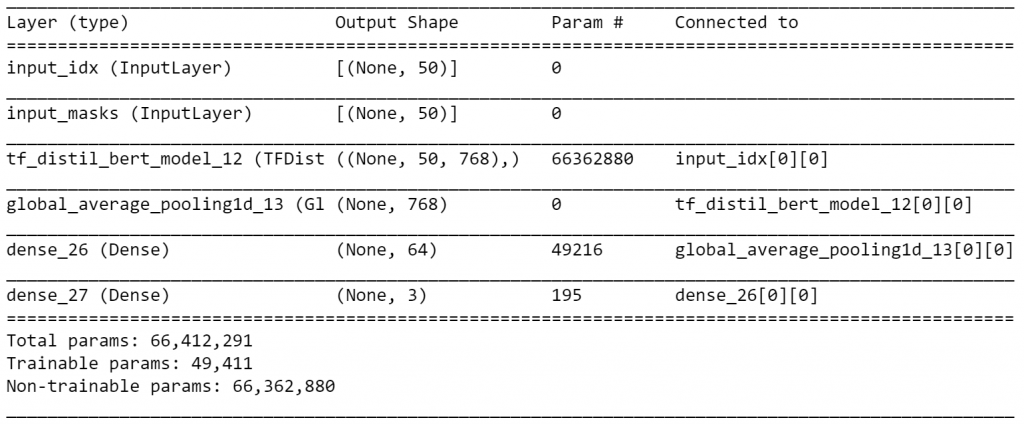
Let’s train, test, evaluate this bad boy (code for evaluation is the same):
## encode y
dic_y_mapping = {n:label for n,label in
                 enumerate(np.unique(y_train))}
inverse_dic = {v:k for k,v in dic_y_mapping.items()}
y_train = np.array([inverse_dic[y] for y in y_train])## train
training = model.fit(x=X_train, y=y_train, batch_size=64,
                     epochs=1, shuffle=True, verbose=1,
                     validation_split=0.3)## test
predicted_prob = model.predict(X_test)
predicted = [dic_y_mapping[np.argmax(pred)] for pred in
             predicted_prob]

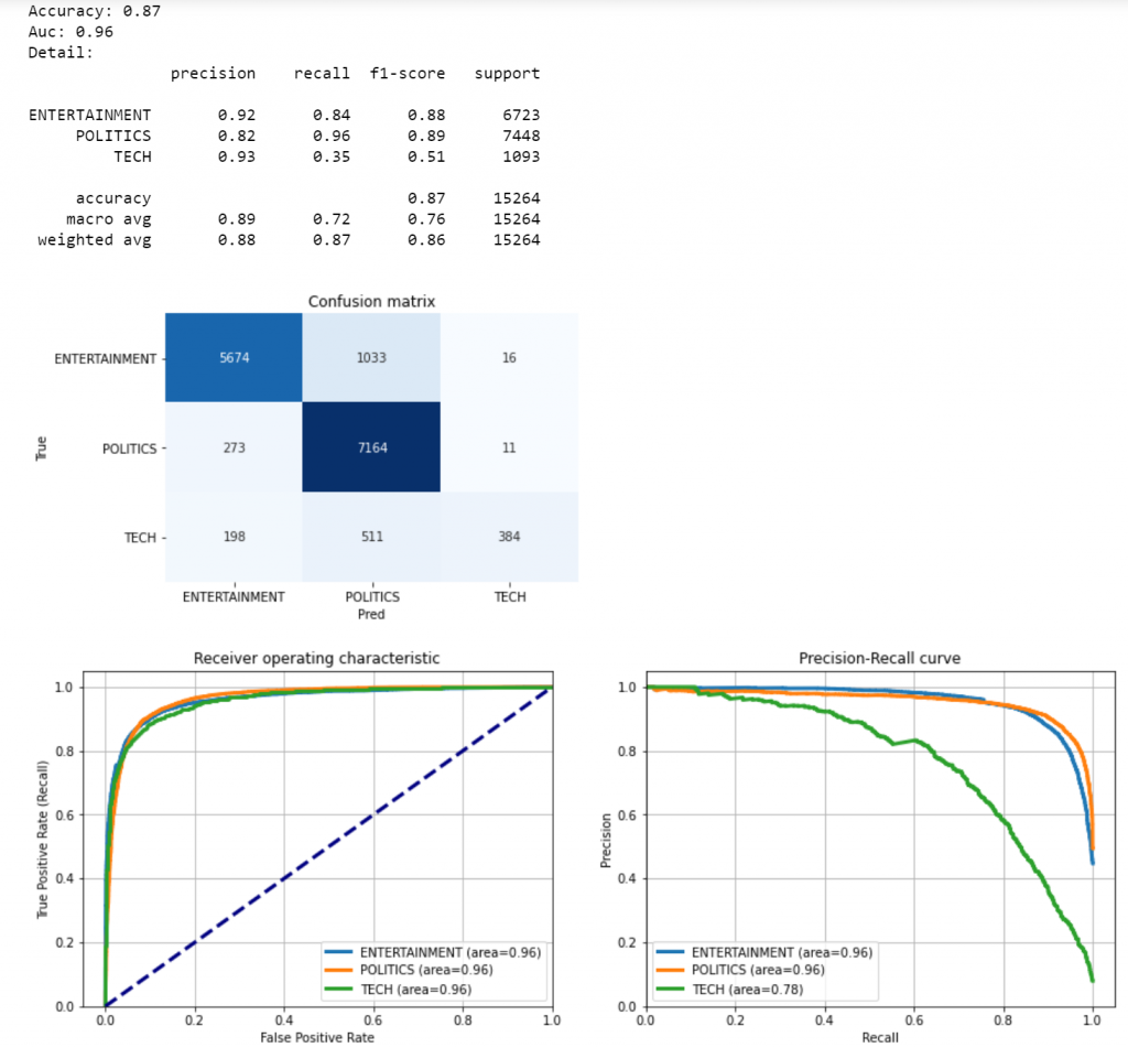
The performance of BERT is slightly better than the previous models, in fact, it can recognize more Tech news than the others.
Conclusion
This article has been a tutorial to demonstrate how to apply different NLP models to a multiclass classification use case. I compared 3 popular approaches: Bag-of-Words with Tf-Idf, Word Embedding with Word2Vec, and Language model with BERT. I went through Feature Engineering & Selection, Model Design & Testing, Evaluation & Explainability, comparing the 3 models in each step (where possible).
Please note that I haven’t covered explainability for BERT as I’m still working on that, but I will update this article as soon as I can. If you have any useful resources about that, feel free to contact me.


