Deep learning on graphs is taking more importance by the day. Here I’ll show the basics of thinking about machine learning and deep learning on graphs with the library Spektral and the platform MatrixDS.
Disclaimer: This is not the second part of the past article on the subject; it’s a continuation of the first part putting the emphasis on deep learning. Read Part 1 here.
Introduction

We are in the process of defining a new way of doing machine learning, focusing on a new paradigm, the data fabric.
In the past article I gave my new definition of machine learning:
Machine learning is the automatic process of discovering hidden insights in data fabric by using algorithms that are able to find those insights without being specifically programmed for that, to create models that solves a particular (or multiple) problem(s).
The premise for understanding this it’s that we have created a data fabric. For me, the best tool out there for me for doing that is Anzo as I mentioned in other articles.
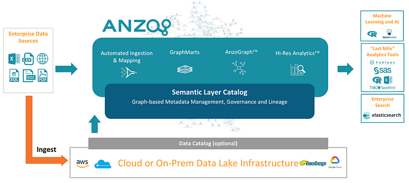
You can build something called “The Enterprise Knowledge Graph” with Anzo, and of course, create your data fabric.
But now I want to focus on a topic inside machine learning, deep learning. In another article I gave a definition of deep learning:
Deep learning is a specific subfield of machine learning, a new take on learning representations from data which puts an emphasis on learning successive “layers” [neural nets] of increasingly meaningful representations.Here we’ll talk about a combination of deep learning and graph theory, and see how it can help move our research forward.
Objectives
General
Set the basis of doing deep learning on the data fabric.Specifics
- Describe the basics of deep learning on graphs.
- Explore the library Spektral.
- Validate the possibility of doing deep learning on the data fabric.
Main Hypothesis
If we can construct a data fabric that supports all the data in the company, the automatic process of discovering insights through learning increasingly meaningful representations from data using neural nets (deep learning) can run inside the data fabric.
Section 1. Deep learning on graphs?
https://tkipf.github.io/graph-convolutional-networks/
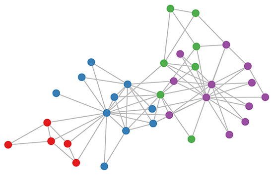
Normally we create neural nets using tensors, but remember that we can also define a tensor with a matrix and graphs can be define through matrices.
In the documentation of the library Spektral they state that a graph is generally represented by three matrices:
- A∈{0,1}#k8SjZc9Dxk(N×N): a binary adjacency matrix, where A_ij=1 if there is a connection between nodes i and j, and A_ij=0 otherwise;
- X∈ℝ#k8SjZc9Dxk(N×F): a matrix encoding node attributes (or features), where an FF-dimensional attribute vector is associated to each node;
- E∈ℝ#k8SjZc9Dxk(N×N×S): a matrix encoding edge attributes, where an S-dimensional attribute vector is associated to each edge.
The important part here is the concept of Graph Neural Networks (GNN).
Graph Neural Networks (GNN)
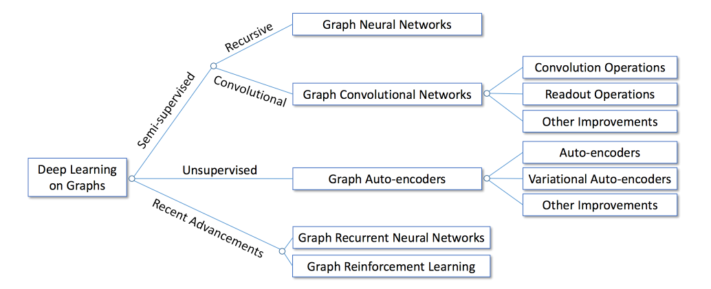
The idea of GNN is simple: to encode structural information of the graph, each node v_i can be represented by a low-dimensional state vector s_i , 1 ≤ i≤ N (Remember vectors can be thought as rank 1 tensors, and tensors can be represented with matrices).
The tasks for learning deep model on graphs can be broadly categorized into two domains:
- Node-focused tasks: the tasks are associated with individual nodes in the graph. Examples include node classification, link prediction and node recommendation.
- Graph-focused tasks: the tasks are associated with the whole graph. Examples includes graph classification, estimating certain properties of the graph or generating graphs.
Section 2. Deep Learning with Spektral

The author defined Spektral as a framework for relational representation learning, built in Python and based on the Keras API.
Installation
The first thing you need to do is to fork the MatrixDS project:
Click on:

you will have the library installed and everything working :).
If you are running this outside remember that the framework is tested for Ubuntu 16.04 and 18.04, and you should install:
sudo apt install graphviz libgraphviz-dev libcgraph6And then install the library with:
pip install spektral
Data representation
In Spektral, some layers and functions are implemented to work on a single graph, while others consider sets (i.e., datasets or batches) of graphs.
The framework distinguishes between three main modes of operation:
- single, where we consider a single graph, with its topology and attributes;
- batch, where we consider a collection of graphs, each with its own topology and attributes;
- mixed, where we consider a graph with fixed topology, but a collection of different attributes; this can be seen as a particular case of the batch mode (i.e., the case where all adjacency matrices are the same) but is treated separately for computational reasons.
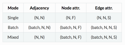
For example, if we run
from spektral.datasets import citation
adj, node_features, edge_features, _, _, _, _, _ = citation.load_data(‘cora’)
We will be loading the data in sigle mode:
Our Adjacency matrix is:
In [3]: adj.shape
Out[3]: (2708, 2708)
Out note attributes are:
In [3]: node_attributes.shape
Out[3]: (2708, 2708)
And our edge attributes are:
In [3]: edge_attributes.shape
Out[3]: (2708, 7)
Semisupervised classification with Graph Attention layers (GAT)
Disclaimer: I’m assuming that you know Keras from here.For more detail and code view:
A GAT is novel neural network architectures that operate on graph-structured data, leveraging masked self-attentional layers. In Spektral the GraphAttention layer computes a convolution similar to
layers.GraphConv, but uses the attention mechanism to weight the adjacency matrix instead of using the normalized Laplacian.
The way they work is by stacking layers in which nodes are able to attend over their neighborhoods’ features, that enables (implicitly) specifying different weights to different nodes in a neighborhood, without requiring any kind of costly matrix operation (such as inversion) or depending on knowing the graph structure upfront.
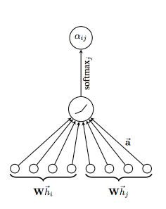
https://arxiv.org/pdf/1812.04202.pdf. The attention mechanism employed by the model, parametrized by a weight vector, applying a LeakyReLU activation.
The model we will use is simple enough:# Layers
dropout_1 = Dropout(dropout_rate)(X_in)
graph_attention_1 = GraphAttention(gat_channels,
attn_heads=n_attn_heads,
attn_heads_reduction=’concat’,
dropout_rate=dropout_rate,
activation=’elu’,
kernel_regularizer=l2(l2_reg),
attn_kernel_regularizer=l2(l2_reg))([dropout_1, A_in])
dropout_2 = Dropout(dropout_rate)(graph_attention_1)
graph_attention_2 = GraphAttention(n_classes,
attn_heads=1,
attn_heads_reduction=’average’,
dropout_rate=dropout_rate,
activation=’softmax’,
kernel_regularizer=l2(l2_reg),
attn_kernel_regularizer=l2(l2_reg))([dropout_2, A_in])
# Build model
model = Model(inputs=[X_in, A_in], outputs=graph_attention_2)
optimizer = Adam(lr=learning_rate)
model.compile(optimizer=optimizer,
loss=’categorical_crossentropy’,
weighted_metrics=[‘acc’])
model.summary()
# Callbacks
es_callback = EarlyStopping(monitor=’val_weighted_acc’, patience=es_patience)
tb_callback = TensorBoard(log_dir=log_dir, batch_size=N)
mc_callback = ModelCheckpoint(log_dir + ‘best_model.h5′,
monitor=’val_weighted_acc’,
save_best_only=True,
save_weights_only=True)
Btw, the model is quite big:
___________________________________________________________________________________
Layer (type) Output Shape Param # Connected to
===============================================================================
input_1 (InputLayer) (None, 1433) 0
___________________________________________________________________________________
dropout_1 (Dropout) (None, 1433) 0 input_1[0][0]
___________________________________________________________________________________
input_2 (InputLayer) (None, 2708) 0
___________________________________________________________________________________
graph_attention_1 (GraphAttenti (None, 64) 91904 dropout_1[0][0]
input_2[0][0]
___________________________________________________________________________________
dropout_18 (Dropout) (None, 64) 0 graph_attention_1[0][0]
___________________________________________________________________________________
graph_attention_2 (GraphAttenti (None, 7) 469 dropout_18[0][0]
input_2[0][0]
===============================================================================
Total params: 92,373
Trainable params: 92,373
Non-trainable params: 0
So if you don’t have that much power lower the number of epochs an play with it. Remember that is very easy to upgrade your MatrixDS account.
Then we train it (this may take some hours if you don’t have enough power):
# Train model
validation_data = ([node_features, adj], y_val, val_mask)
model.fit([node_features, adj],
y_train,
sample_weight=train_mask,
epochs=epochs,
batch_size=N,
validation_data=validation_data,
shuffle=False, # Shuffling data means shuffling the whole graph
callbacks=[es_callback, tb_callback, mc_callback])
Get the best model:
model.load_weights(log_dir + 'best_model.h5')
And evaluate it:
print(‘Evaluating model.’)
eval_results = model.evaluate([node_features, adj],
y_test,
sample_weight=test_mask,
batch_size=N)
print(‘Done.
‘
‘Test loss: {}
‘
‘Test accuracy: {}’.format(*eval_results))
See more in the MatrixDS project:
MatrixDS | The Data Project Workbench
MatrixDS is a place to build, share and manage data projects at any scale.community.platform.matrixds.com
Section 3. Where does this fit in the data fabric?
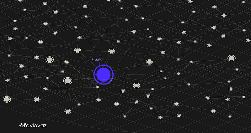
If you remember from the last part that if we have a data fabric:
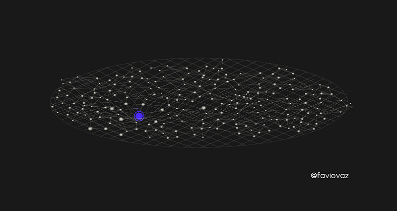
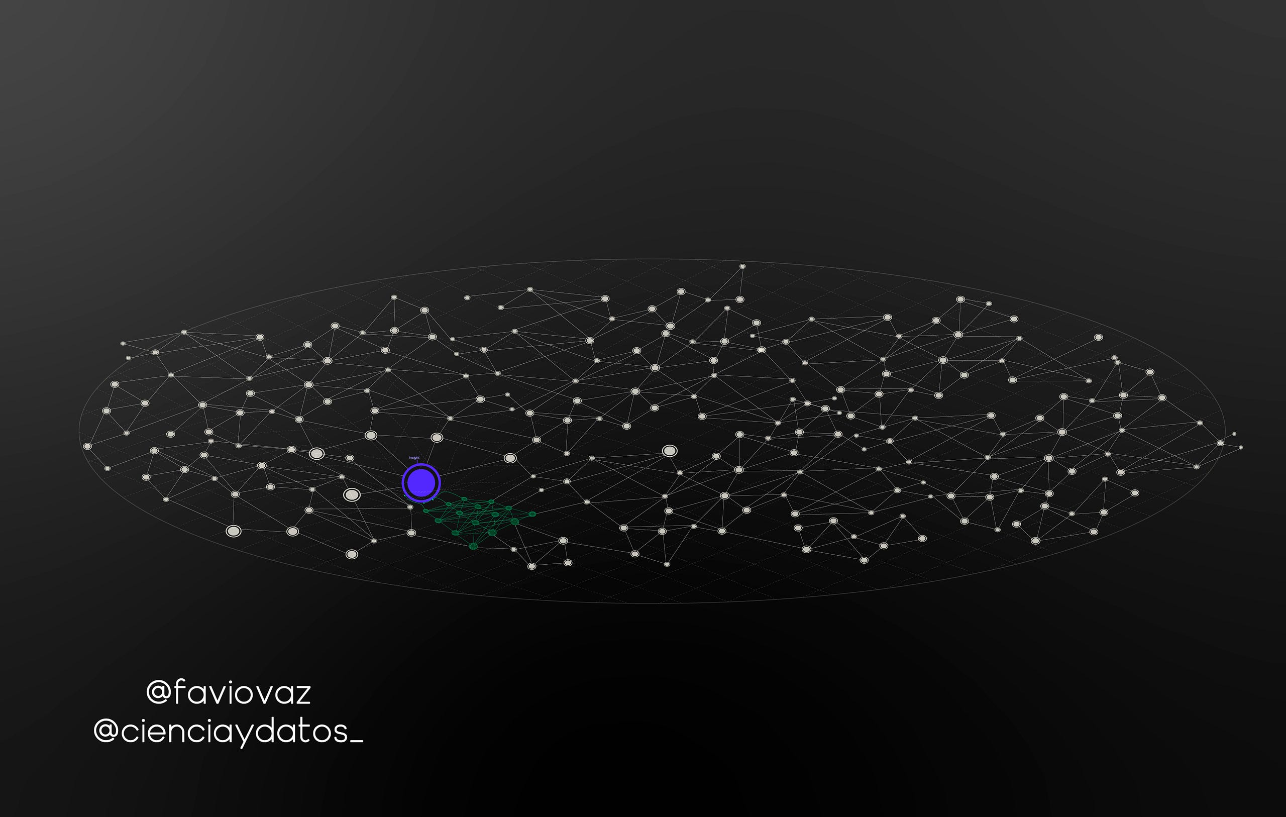
An insight can be thought of as a dent in it:
And if you are following this tutorial in the MatrixDS platform, you realized that the data we are using is not a simple CS, but we provided the library with:
- an N by N adjacency matrix (N is the number of nodes),
- an N by D feature matrix (D is the number of features per node), and
- an N by E binary label matrix (E is the number of classes).
And that was stored is a series of files:
ind.dataset_str.x => the feature vectors of the training instances as scipy.sparse.csr.csr_matrix object; ind.dataset_str.tx => the feature vectors of the test instances as scipy.sparse.csr.csr_matrix object; ind.dataset_str.allx => the feature vectors of both labeled and unlabeled training instances (a superset of ind.dataset_str.x) as scipy.sparse.csr.csr_matrix object; ind.dataset_str.y => the one-hot labels of the labeled training instances as numpy.ndarray object; ind.dataset_str.ty => the one-hot labels of the test instances as numpy.ndarray object; ind.dataset_str.ally => the labels for instances in ind.dataset_str.allx as numpy.ndarray object; ind.dataset_str.graph => a dict in the format {index: [index_of_neighbor_nodes]} as collections.defaultdict object; ind.dataset_str.test.index => the indices of test instances in graph, for the inductive setting as list object.
So this data lives in a graph. And what we did was loading that data to the library. Actually, you can transform your data from and to NetworkX, numpy and sdf format in the library.
This means, that if we are storing our data in a data fabric, we have our knowledge-graph so we already have a lot of these features, what we have is to find a way of connecting it with the library. That’s the tricky part right now.
And then we can start finding insights in your data fabrics through the process of running deep learning algorithms on the graphs inside of it.The interesting part here is that there could be ways of running these algorithms in the graph itself, and for that we need to be able to build models with data stored inherently in the graph’s structure, there’s a very interesting approach for that with Neo4j by Lauren Shin here:
But it’s also a work in progress. I imagine the process to be something like this:

Meaning that the neural net could live inside the data fabric, and the algorithms will be running with the resources inside it.
One important thing I’m not even mentioning here is the concept of non-euclidean data but I’ll go there later.
Conclusions
It’s possible to run deep learning algorithms on the data fabric by deploying graph neural nets models for the graph data we have if we can connect the knowledge-graph with the Spektral (or other) library.
Besides standard graph inference tasks such as node or graph classification, graph-based deep learning methods have also been applied to a wide range of disciplines, such as modeling social influence, recommendation systems, chemistry, physics, disease or drug prediction, natural language processing (NLP), computer vision, traffic forecasting, program induction and solving graph-based NP problems. See https://arxiv.org/pdf/1812.04202.pdf.
The applications are endless, this is the beginning of a new exciting era. Stay tuned for more 🙂


