What are the challenges posing data scientists and how are researchers tackling them?
“The human brain uses much less energy than a computer, yet it is infinitely more complex and intricate.” — Nayef Al-Rodhan, Global Policy Journal
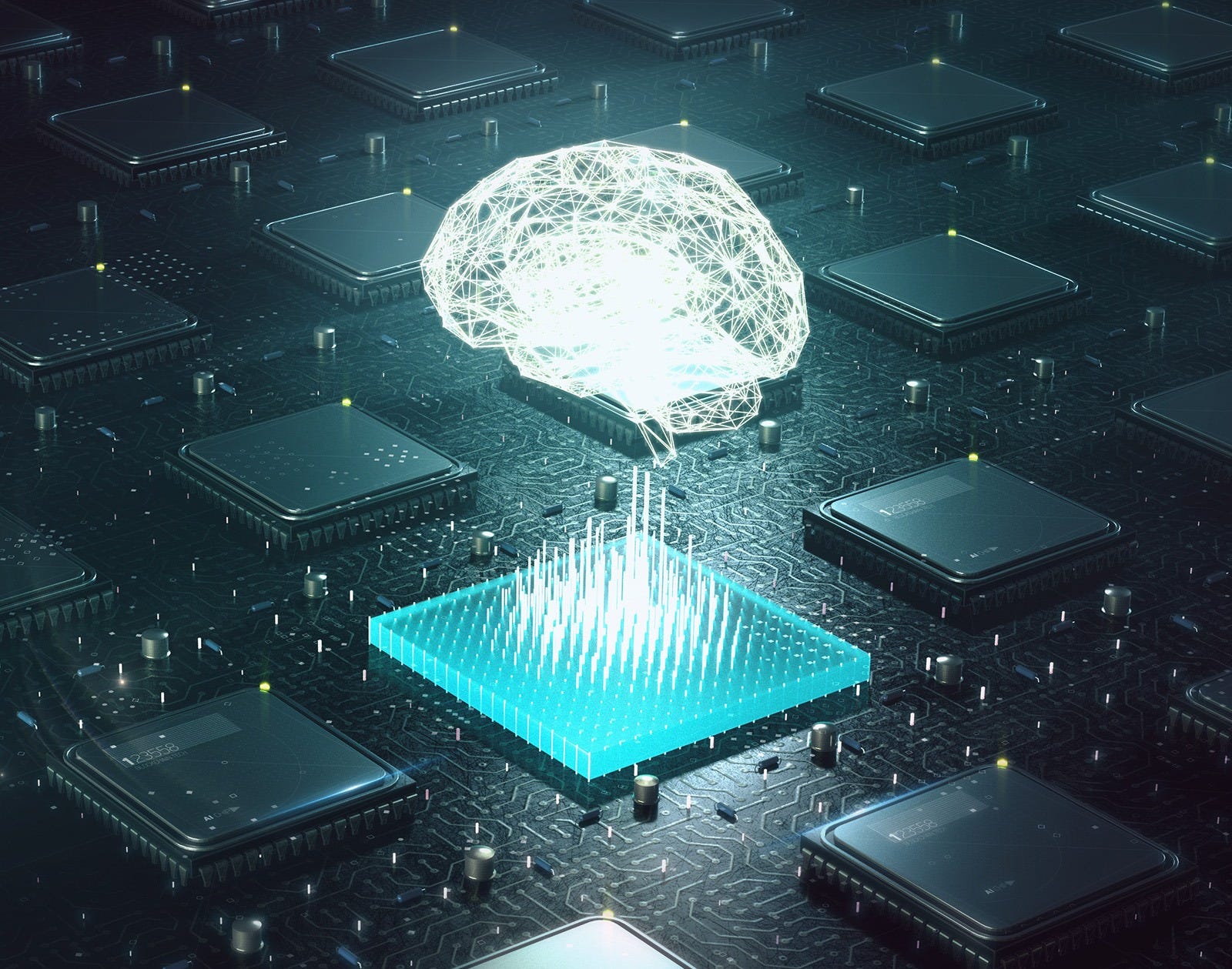
Source: https://www.nanalyze.com/2019/08/neuromorphic-computing-ai-chip/
In this article, I will discuss the current challenges and expected future trends in computational science with a bent towards their impacts on the fields of data science and machine learning. This includes the breakdown of Dennard scaling — the slowdown of Moore’s law, the burgeoning field of the internet of things (IoT), and the advent of more energy-efficient computing that mimics the human brain, known as neuromorphic computing.
The Trends
Deep Learning
Deep learning has become ubiquitous in the modern world, with wide-ranging applications in nearly every field. As might be expected, people have started to notice, and the hype behind deep learning continues to increase as its widespread adoption by businesses occurs. Deep learning consists of neural networks with multiple hidden layers and has some particularly demanding needs in terms of computational resources:
- 1 billion parameters to train.
- Computational intensity increases as the network depth grows
Deep learning has been hugely successful for some important tasks in speech recognition, computer vision, and text understanding.
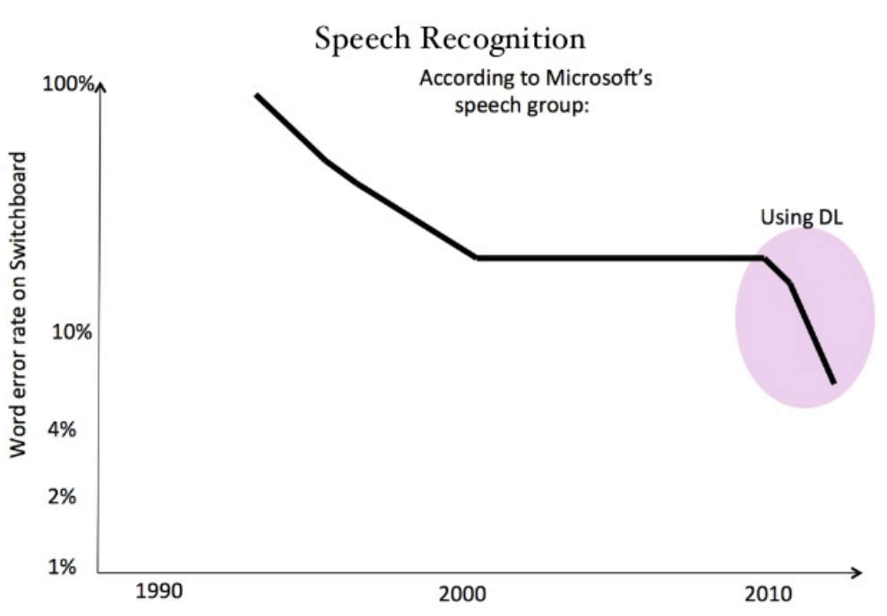
The apparent success of deep learning in the field of speech recognition
The major downside of deep learning is its computational intensity, requiring high-performance computational resources and long training times. For facial recognition and image reconstructions, this also means working with low-resolution images. How will researchers aim to tackle these big compute problems? And what is the bottleneck of this approach in the first place?
Internet of Things (IoT)
A total of 20 billion embedded devices are expected to be active in the next several years, stemming from smart fridges, phones, thermostats, air quality sensors, locks, dog collars, the list is impressively long. Most of these devices will be battery powered and severely resource-constrained in memory and computing power. In spite of these limitations, these devices need to perform intelligent tasks and be easy to use.
The expected prevalence of IoT devices comes with major concerns, particularly regarding the security of these devices (perhaps future criminals will be hackers that can hack my smart locks on my doors). It also portends the advent of data-driven deep learning. Deep learning already requires extensive amounts of data, but the presence of large-scale networked devices or sensors opens new avenues of research — especially in my own field of environmental science, which is seeing an increasing push towards low-cost and large-scale sensor networks to monitor atmospheric pollutants.
This idea also extends to smartphones. Smartphones are becoming increasingly powerful and now rival some old laptops in their computational abilities. Increasingly, machine learning is performed on these devices. Despite their improvements, they are still limited in their computational resources and hence trends towards reducing computational and data overhead are increasingly important on these devices.
This idea also extends to self-driving cars, which are beginning to be commercialized after a long period of research and development. Self-driving cars present their own issues but still suffer from the same concerns, the most publicized of which are the security and ethical underpinning of the vehicles.
More data means more data science (woohoo for the data scientists!), but it also means needing to store and process this data, and to transmit this data through wireless networks (and do it securely, I might add). How are the problems associated with IoT to be tackled? And whose responsibility is it if something goes wrong?
Cloud-Based Computing
There is an increasing push towards the use of cloud computing by companies in order to outsource their computational needs and minimize costs.
This also aids companies (especially startups) by reducing capital costs associated with purchasing infrastructure and instead moving it to operating costs. With the growing popularity of machine learning and data science, which are computationally intensive and require high-performance systems, as well as the increasing online presence of most corporations, this trend in cloud-based distributed computing is not expected to slow down anytime soon.
Scaling Computation Size
Scaling up computation size with only modestly increased energy consumption is a difficult task. We need such balanced computation scaling for deep neural networks to minimize their energy overhead.
The current solution of this is the parallel use of many small, energy-efficient compute nodes to accommodate large computations.
Reducing Energy Usage
Scaling down energy with only modestly decreased outcome quality (e.g., prediction accuracy) is becoming an increasingly important task. We need such balanced energy scaling for IoT devices and wearables. These considerations are related to a new field called approximate computing which trades off quality with the effort expended.
The current solution to this is the coordinated use of multiple small, energy-efficient compute nodes to support intelligent computations.
More Data
The data trend is clearly not going to stop any time soon! However, a discussion for this deserves its own section.
Data Overload
The data explosion of the past two decades now means that humanity produces the same amount of data as all of mankind up to 2003, every 2 days. Computing trends show that we are now in the region of exascale data, which refers to the computing of data on the scale of 1 billion gigabytes, as well as exascale computing, which refers to computers capable of performing 10¹⁸ computations per second.
The sum total of data held by all the big online storage and service companies like Google, Amazon, Microsoft and Facebook make up about 4,800 petabytes (4.8 Exabytes).
Analyzing large sets of data (even a few gigabytes) requires different approaches to running models on your local laptop — trying to do so will simply crash your computer.
Parallelization
Currently the standard ways of processing highly expensive computations, which are typically done with supercomputers (for big compute tasks, requiring lots of computing power), or with large distributed systems (for big data tasks, that require lots of computational memory).
In the near future, if you want to analyze large data sets, you will essentially have no choice but to turn to parallel computing.
Distributed systems work well up to a point, but quickly break down once we approach clusters (a group of computers working on a single task) with 1,000 nodes (individual computers in a cluster). Most of the time in the cluster is spent communicating, which causes overheads that slow down the overall computation of a system. This phenomenon is known as parallel slowdown.
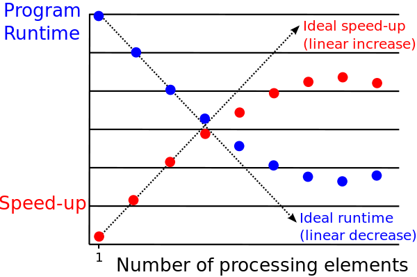
Illustration of parallel slowdown — initially, we see an improvement in the speedup as the number of processors increases. This relationship breaks down for large numbers of processing elements due to a communications bottleneck (too many people talking, not enough work being done). Source
Another compounding issue we run into is the proportion of our computation that is parallelizable, which is described by Amdahl’s Law:
Amdahl’s law states that in parallelization, if P is the proportion of a system or program that can be made parallel, and 1-P is the proportion that remains serial, then the maximum speedup that can be achieved using N number of processors is 1/((1-P)+(P/N)).
In layman’s term, our maximum speedup depends on the proportion of the program that must be done sequentially — the proportion that is not parallelizable. If 50% of our computation is parallelizable, we can get much less speedup than if our program is 95% parallelizable. This phenomenon is illustrated below.
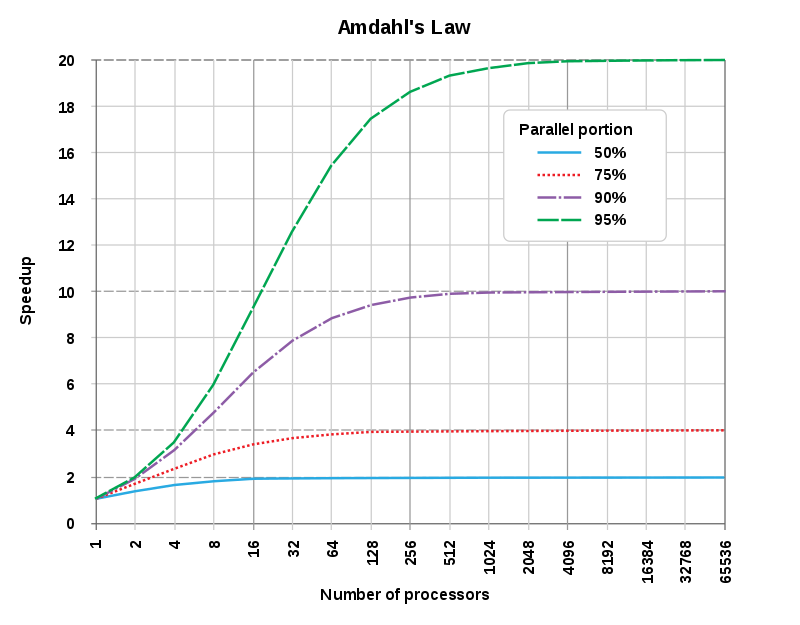
Amdahl’s law, illustrated. As the number of processors we have available increases, we reach a bottleneck which depends on the serial portion of our algorithm. Source
This problem disappears for computations that are embarrassingly parallel, which means that the program is 100% parallelizable and essentially separate — for example, testing of different hyperparameters of a neural network.
Note: What is the difference between parallel computing and distributed computing? Parallel computing is the simultaneous use of multiple compute nodes over shared memory. Distributed computing is the simultaneous use of multiple compute nodes each working on their own memory.
Distributed computing systems that underpin the online systems of many businesses are commonly seen on the cloud nowadays, with business offloading most of their computational infrastructure to big cloud companies such as Amazon and Microsoft for easier and cheaper maintenance.
Supercomputers work well but they are extremely expensive to run and maintain, and they are in high demand. Within universities such as Harvard, labs have access to a proportion of the computational resources, which can be shared among the group members. However, rental costs are very expensive. In the field of environmental science, running a global climate model for a month with an hourly time resolution can take several weeks to run, which can be extremely costly.
Computing power has always been an issue, but nowadays the biggest issue is that the data we have is just getting too big to handle. Even if we assume Moore’s law still to hold (which is discussed in the next section), data production is exponential whereas Moore’s law is linear. The amount of data available to process quickly incapacitates any general-purpose computer, or set of computers configured together in a cluster if the computational intensity is large enough.
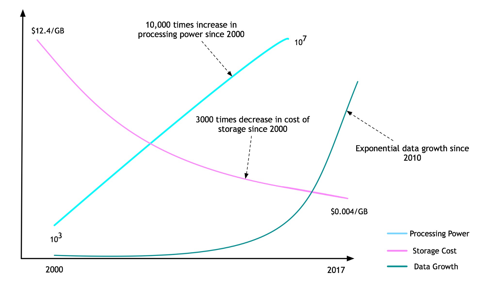
Computing trends in processing power, storage cost, and data growth. Source
Cloud computing is not cheap if you have a thousand computers running at once to manage your business’ database servers, but at least it is feasible. How, on the other hand, would you expect to perform business analytics on a dataset that is 100 Petabytes? Disk space is incredibly cheap, but memory is not, and your data must be in memory before it can be readily analyzed.
Fortunately, we can at least estimate how long a computation (which can also be extended to data) might take by something called the wall clock time. This can be done by first finding the computational complexity of your computation:
CC = CD*N *T
- CC = computational complexity (# Flops)
- CD = computational density (# Flops/site/step)
- N = Domain size or number of data points (# sites)
- T = Number of timesteps or epochs (# steps)
To calculate the wall clock time, you need to know the processing power of your laptop (e.g. 1 GFlops/s). Then:
WCT = CC / processing power
For example, if you are performing a computation on a 2D grid with 1000 data points for 1000 timesteps, you will perform 6 computations at each grid point. This has a computational intensity of 6 ExaFlops, which will take you about 6000 seconds (~2 hours) on a 1 GFlops/s laptop.
For a list of computational complexities for a variety of different machine learning algorithms, see the table below.
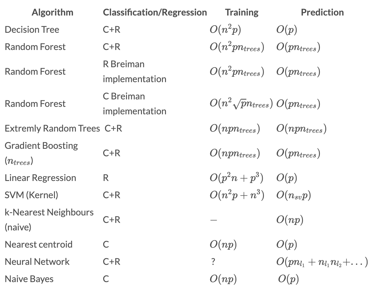
Computational complexities of machine learning algorithms. Source
Estimate your wall clock time before you do a large computation!
As can be seen, the time increases in proportional to the number of computations, which is related to (1) the number of data points, or (2) the size of the computational domain.
How important is parallelization within machine learning? Extremely important, as it turns out. There are two ways this can occur:
- Data parallelism — distribute data, use the same model.
- Model parallelism — distribute model, use the same data.
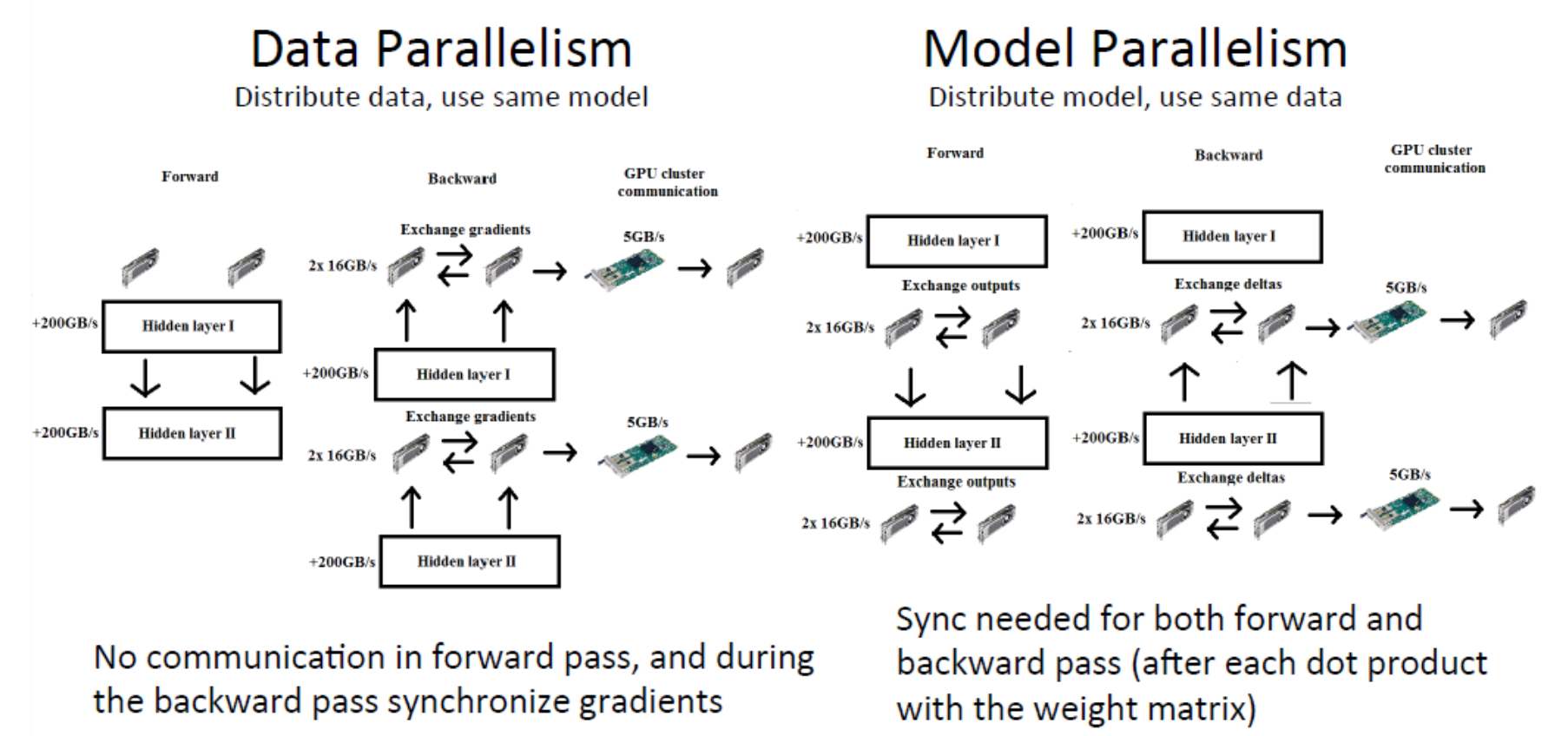
Data parallelism vs model parallelism
How do people expect to handle the increasingly huge amount of data that must be analyzed? There are a number of options, although this is by means exhaustive:
[1] Instead of moving the ‘compute’ to the data, move the data to the ‘compute’. There is a big push for this in the environmental sciences due to the presence of large-scale distributed networks.
- Edge and fog computing — where computations are done closer to the data sources on edge devices. This will become important in the IoT infrastructure.
[2] Hierarchical segmentation of workloads to produce non-interactive workloads that can be distributed (not always possible for interactive workloads).
- Grid computing — imagine performing hyperparameter tuning on a neural network and sending one set of hyperparameters to one computational cluster, and another set to a second cluster (an example of model parallelism). The two clusters do not communicate and are effectively independent. This is not (typically) feasible for data parallelism in a neural network, for example.
[3] Improvements in high-speed communication, parallel frameworks, or time management of distributed systems (these are already pretty good though!).
[4] Using specialized hardware such as ASICs (like people have done for bitcoin mining, to optimize hardware for a specific computation), GPUs, and TPUs. One GPU can provide the performance of 8 CPUs on graphical data, and a single TPU can be as effective as 8 GPUs — naturally, they do not come cheap.
How can I implement parallelization in my own work?
Speed is becoming increasingly important for computation due to the need to analyze huge datasets in a tractable timeframe. Python is an excellent language that is the most popular language used by data scientists, but sadly it is not a particularly fast language (for one thing, it is interpreted and not compiled, which means the code is translated into binary code on-the-fly, which takes additional time).
Parallelization is possible in most languages in order to speed up the code, and this can be in the form of adding extra processors, as we have discussed, or by using additional threads — if you are not familiar, think of this as opening two of the same computer program such that they can share the program load. This is known as multithreading, and whilst less useful for massive datasets, it can still provide a substantial benefit. One of the most popular implementations of this is OpenMP for use in C++.
Multithreading is an important issue with Python, due to something called the GIL. We cannot use OpenMP but, fortunately, there is a multithreading library imaginatively called multithreading that can be used.
Parallelization between processors can be done using MPI, and can be extended to graphical processing units (GPUs) and also more specialized equipment (such as Google’s Tensor Processing Unit) using other parallel frameworks such as OpenACC. These are reasonably easy to set up on instances offered by cloud providers (TPUs are only offered by GoogleCloud).
If working with images, I highly recommend doing computations with at the very least one GPU. This can reduce training times by an order of magnitude — that is the difference between waiting an hour and an entire day.
The End of Moore’s Law (as we know it)
In 1965, Gordon Moore, an Intel co-founder, made a prediction that would set the pace for our modern digital revolution. From careful observation of an emerging trend, Moore extrapolated that computing would dramatically increase in power, and decrease in relative cost, at an exponential pace.
But slower pace is expected in the future. In July 2015 Intel CEO Brian Krzanich said, “the exponential advances in semiconductor manufacturing that enable faster and cheaper computing and storage every two years are now going to come closer to a rate of every two and half years”.
Rather than continuing to make microprocessors more and more powerful, people now work on new architectures and computing models which leverage parallel processing to provide balanced computation and energy scaling, as noted earlier.
Moore’s law — the phenomenon that the number of transistors on a CPU doubles around every 2 years — is still observed to some extent, but the assumption that computing power still scales exactly with the area has been seen to have broken down. This assumption of the scaling of power density is known as Dennard scaling.
Dennard scaling states, roughly, that as transistors get smaller their power density stays constant, so that the power use stays in proportion with area: both voltage and current scale (downward) with length.
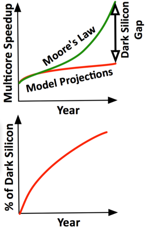
Source: Dark Silicon and the End of Multicore Scaling, 2011.
Since around 2005–2007, Dennard scaling appears to have broken down, so even though Moore’s law continued for several years after that, it has not yielded dividends in improved performance. The primary reason cited for the breakdown is that at small sizes, current leakage poses greater challenges, and also causes the chip to heat up.
There have been diverse approaches to heat management, from pumping Fluorinert through the system, to a hybrid liquid-air cooling system or air cooling with normal air conditioning temperatures. However, these approaches only work up to a point, and after this the only thing that can be done is to select parts of the chip to power on.
Because of this, sections of the chip sometimes are not powered-on in order to keep the chip temperature in the safe operating range. These regions are referred to as dark silicon.
Designs are needed that can dynamically select parts of the chip to power on — this is an active area of computational research that will become increasingly important as time passes and Moore’s law continues to deviate from its original predictions.
Neuromorphic Computing
Neuromorphic computing is the development of computing systems that mimic the neurobiological architectures present in the nervous system.
A key aspect of neuromorphic engineering is understanding how the morphology of individual neurons, circuits, applications, and overall architectures creates desirable computations, affects how information is represented, influences robustness to damage, incorporates learning and development, adapts to local change (plasticity), and facilitates evolutionary change.
Morphic is defined as in a specific shape or form. Neuromorphic means having behaviors of neurons.
In a conference proceeding to the IEEE in 1990 titled Neuromorphic Electronic Systems, the concept of neuromorphic computing was first introduced. The proceedings stated that:
“The human brain has 10¹⁶ synapses, with a nerve pulse arriving at each synapse per 100ms. This means 10¹⁶ complex operations per second. At the power dissipation of 1W (instead of 20W for simplicity here), the brain does each operation only 1/10¹⁶ J — In contrast, the ultimate silicon technology will dissipate 1/10⁹ J for each operation.”
Thus, it is expected that by implementing neuromorphic computing, we may be able to achieve computations that are orders of magnitude more energy-efficient than our current systems.
The push towards energy-efficient computing comes about for multiple reasons, not just for reducing costs — although that is a reason. This also frees up computations for hardware, allowing the same number of computations to be done on fewer devices, which have cost benefits as well as potential benefits to parallelization. There are also clear environmental benefits to reducing the total energy consumption of devices.
There are many examples of early efforts in neuromorphic computing:
- Neurogrid is a multi-chip system developed by Kwabena Boahen and his group at Stanford, 2005 (6,000 synapses).
- Fast Analog Computing with Emergent Transient States (FACETS), 2005 (50 million synapses).
- Torres-Huitzil’s FPGA Model, 2005.
One of the latest efforts is IBM’s TrueNorth. The TrueNorth consumes about 1/10¹³ J per operation, rather than 1/10⁹ J in general-purpose computing. Recall that for human brain this number is 1/10¹⁶ J. Thus we still have three orders of magnitude to go!
Final Comments
In summary, the future of computation looks like it will involve speeding up computations to handle the relentless and exponential increase in data production. However, speeding up individual processors is difficult for various reasons, and Moore’s law cannot last forever — it is becoming increasingly constrained by the limits of heat transfer and quantum mechanics. A greater push will continue to be seen towards parallel computing, especially with more specialized hardware such as GPUs and TPUs, as well as towards more energy-efficient computing which may become possible as we enter into the realm of neuromorphic computing.
The burgeoning area of IoT devices presents different challenges, which are trying to be challenged using more compute-central ideas such as edge and fog computing.
Disclaimer: I left out quantum computing out of this article as it is not clear to me that this is likely to be a feasible computational option anytime in the near future.
Further Topics
There are various other topics that are worthy of note for the interested reader. I recommend looking more into these if they pique your interest, they may become important in the near future:
- Automata processors
- Neuromorphic spike-based computing
- AI Accelerators
- Heterogeneous computing
References
Monroe, D. (2014). “Neuromorphic computing gets ready for the (really) big time”. Communications of the ACM. 57 (6): 13–15. doi:10.1145/2601069
Modha, Dharmendra (August 2014). “A million spiking-neuron integrated circuit with a scalable communication network and interface”. Science. 345 (6197): 668–673.
Mead, Carver (1990). “Neuromorphic electronic systems” (PDF). Proceedings of the IEEE. 78 (10): 1629–1636. doi:10.1109/5.58356
Amdahl, Gene M. (1967). “Validity of the Single Processor Approach to Achieving Large-Scale Computing Capabilities” (PDF). AFIPS Conference Proceedings (30): 483–485. doi:10.1145/1465482.1465560.
Rodgers, David P. (June 1985). “Improvements in multiprocessor system design”. ACM SIGARCH Computer Architecture News. New York, NY, USA: ACM. 13 (3): 225–231. doi:10.1145/327070.327215. ISBN 0–8186–0634–7. ISSN 0163–5964
Dennard, Robert H.; Gaensslen, Fritz; Yu, Hwa-Nien; Rideout, Leo; Bassous, Ernest; LeBlanc, Andre (1974). “Design of ion-implanted MOSFET’s with very small physical dimensions” (PDF). IEEE Journal of Solid-State Circuits. SC-9 (5).
Greene, Katie (2011). “A New and Improved Moore’s Law: Under “Koomey’s law,” it’s efficiency, not power, that doubles every year and a half”. Technology Review.
Bohr, Mark (2007). “A 30 Year Retrospective on Dennard’s MOSFET Scaling Paper” (PDF). Solid-State Circuits Society. Retrieved January 23, 2014.
Esmaeilzedah, Hadi; Blem, Emily; St. Amant, Renee; Sankaralingam, Kartikeyan; Burger, Doug (2012). “Dark Silicon and the end of multicore scaling” (PDF).
Hruska, Joel (2012). “The death of CPU scaling: From one core to many — and why we’re still stuck”. ExtremeTech. Retrieved January 23, 2014.

