Interest in machine learning has exploded over the past decade. You see machine learning in computer science programs, industry conferences, and the Wall Street Journal almost daily. For all the talk about machine learning, many conflate what it can do with what they wish it could do. Fundamentally, machine learning is using algorithms to extract information from raw data and represent it in some type of model. We use this model to infer things about other data we have not yet modeled.
Neural networks are one type of model for machine learning; they have been around for at least 50 years. The fundamental unit of a neural network is a node, which is loosely based on the biological neuron in the mammalian brain. The connections between neurons are also modeled on biological brains, as is the way these connections develop over time (with “training”).
In the mid-1980s and early 1990s, many important architectural advancements were made in neural networks. However, the amount of time and data needed to get good results slowed adoption, and thus interest cooled. In the early 2000s, computational power expanded exponentially and the industry saw a “Cambrian explosion” of computational techniques that were not possible prior to this. Deep learning emerged from that decade’s explosive computational growth as a serious contender in the field, winning many important machine learning competitions. The interest has not cooled as of 2017; today, we see deep learning mentioned in every corner of machine learning.
There is an abundant amount of great knowledge about deep learning I have learnt via research and learning. Here I want to share the 10 powerful deep learning methods AI engineers can apply to their machine learning problems. But first of all, let’s define what deep learning is. Deep learning has been a challenge to define for many because it has changed forms slowly over the past decade. To set deep learning in context visually, the figure below illustrates the conception of the relationship between AI, machine learning, and deep learning.
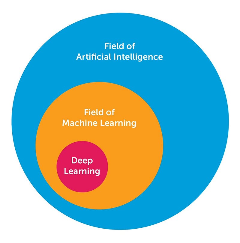
The field of AI is broad and has been around for a long time. Deep learning is a subset of the field of machine learning, which is a subfield of AI. The facets that differentiate deep learning networks in general from “canonical” feed-forward multilayer networks are as follows:
- More neurons than previous networks
- More complex ways of connecting layers
- “Cambrian explosion” of computing power to train
- Automatic feature extraction
When I say “more neurons”, I mean that the neuron count has risen over the years to express more complex models. Layers also have evolved from each layer being fully connected in multilayer networks to locally connected patches of neurons between layers in Convolutional Neural Networks and recurrent connections to the same neuron in Recurrent Neural Networks (in addition to the connections from the previous layer).
Deep learning then can be defined as neural networks with a large number of parameters and layers in one of four fundamental network architectures:
- Unsupervised Pre-trained Networks
- Convolutional Neural Networks
- Recurrent Neural Networks
- Recursive Neural Networks
In this post, I am mainly interested in the latter 3 architectures. A Convolutional Neural Network is basically a standard neural network that has been extended across space using shared weights. CNN is designed to recognize images by having convolutions inside, which see the edges of an object recognized on the image. A Recurrent Neural Network is basically a standard neural network that has been extended across time by having edges which feed into the next time step instead of into the next layer in the same time step. RNN is designed to recognize sequences, for example, a speech signal or a text. It has cycles inside that implies the presence of short memory in the net. A Recursive Neural Network is more like a hierarchical network where there is really no time aspect to the input sequence but the input has to be processed hierarchically in a tree fashion. The 10 methods below can be applied to all of these architectures.
1 — Back-Propagation
Back-prop is simply a method to compute the partial derivatives (or gradient) of a function, which has the form as a function composition (as in Neural Nets). When you solve an optimization problem using a gradient-based method (gradient descent is just one of them), you want to compute the function gradient at each iteration.
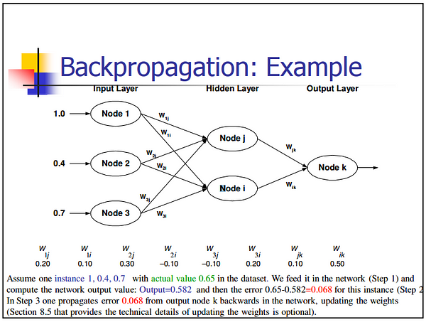
For a Neural Nets, the objective function has the form of a composition. How do you compute the gradient? There are 2 common ways to do it: (i) Analytic differentiation. You know the form of the function. You just compute the derivatives using the chain rule (basic calculus). (ii) Approximate differentiation using finite difference. This method is computationally expensive because the number of function evaluation is O(N), where N is the number of parameters. This is expensive, compared to analytic differentiation. Finite difference, however, is commonly used to validate a back-prop implementation when debugging.
2 — Stochastic Gradient Descent
An intuitive way to think of Gradient Descent is to imagine the path of a river originating from top of a mountain. The goal of gradient descent is exactly what the river strives to achieve — namely, reach the bottom most point (at the foothill) climbing down from the mountain.
Now, if the terrain of the mountain is shaped in such a way that the river doesn’t have to stop anywhere completely before arriving at its final destination (which is the lowest point at the foothill, then this is the ideal case we desire. In Machine Learning, this amounts to saying, we have found the global mimimum (or optimum) of the solution starting from the initial point (top of the hill). However, it could be that the nature of terrain forces several pits in the path of the river, which could force the river to get trapped and stagnate. In Machine Learning terms, such pits are termed as local minima solutions, which is not desirable. There are a bunch of ways to get out of this (which I am not discussing).
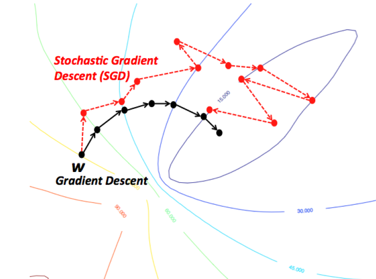
Gradient Descent therefore is prone to be stuck in local minimum, depending on the nature of the terrain (or function in ML terms). But, when you have a special kind of mountain terrain (which is shaped like a bowl, in ML terms this is called a Convex Function), the algorithm is always guaranteed to find the optimum. You can visualize this picturing a river again. These kind of special terrains (a.k.a convex functions) are always a blessing for optimization in ML. Also, depending on where at the top of the mountain you initial start from (ie. initial values of the function), you might end up following a different path. Similarly, depending on the speed at the river climbs down (ie. the learning rate or step size for the gradient descent algorithm), you might arrive at the final destination in a different manner. Both of these criteria can affect whether you fall into a pit (local minima) or are able to avoid it.
3 — Learning Rate Decay
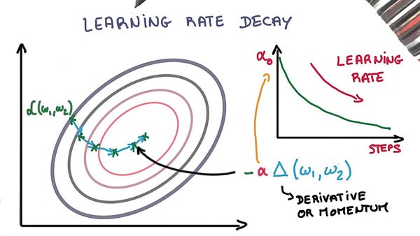
Adapting the learning rate for your stochastic gradient descent optimization procedure can increase performance and reduce training time. Sometimes this is called learning rate annealing or adaptive learning rates. The simplest and perhaps most used adaptation of learning rate during training are techniques that reduce the learning rate over time. These have the benefit of making large changes at the beginning of the training procedure when larger learning rate values are used, and decreasing the learning rate such that a smaller rate and therefore smaller training updates are made to weights later in the training procedure. This has the effect of quickly learning good weights early and fine tuning them later.
Two popular and easy to use learning rate decay are as follows:
- Decrease the learning rate gradually based on the epoch.
- Decrease the learning rate using punctuated large drops at specific epochs.
4 — Dropout
Deep neural nets with a large number of parameters are very powerful machine learning systems. However, overfitting is a serious problem in such networks. Large networks are also slow to use, making it difficult to deal with overfitting by combining the predictions of many different large neural nets at test time. Dropout is a technique for addressing this problem.
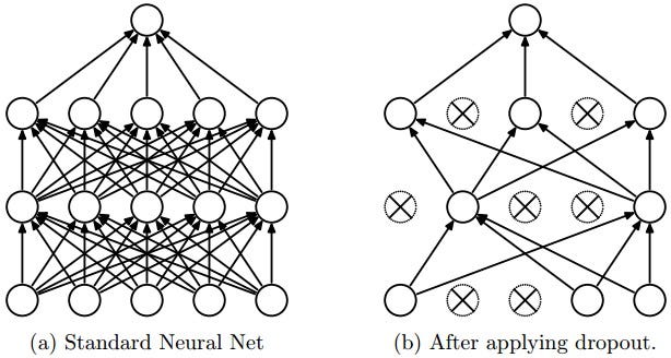
The key idea is to randomly drop units (along with their connections) from the neural network during training. This prevents units from co-adapting too much. During training, dropout samples from an exponential number of different “thinned” networks. At test time, it is easy to approximate the effect of averaging the predictions of all these thinned networks by simply using a single untwined network that has smaller weights. This significantly reduces overfitting and gives major improvements over other regularization methods. Dropout has been shown to improve the performance of neural networks on supervised learning tasks in vision, speech recognition, document classification and computational biology, obtaining state-of-the-art results on many benchmark datasets.
5 — Max Pooling
Max pooling is a sample-based discretization process. The object is to down-sample an input representation (image, hidden-layer output matrix, etc.), reducing its dimensionality and allowing for assumptions to be made about features contained in the sub-regions binned.
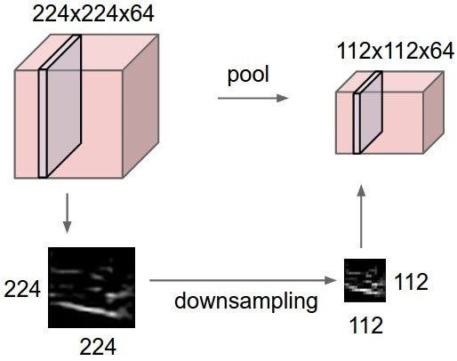
This is done in part to help over-fitting by providing an abstract form of the representation. As well, it reduces the computational cost by reducing the number of parameters to learn and provides basic translation invariance to the internal representation. Max pooling is done by applying a max filter to usually non-overlapping subregions of the initial representation.
6 — Batch Normalization
Naturally, neural networks including deep networks require careful tuning of weight initialization and learning parameters. Batch normalization helps relaxing them a little.
Weights problem:
- Whatever the initialization of weights, be it random or empirically chosen, they are far away from the learned weights. Consider a mini batch, during initial epochs, there will be many outliers in terms of required feature activations.
- The deep neural network by itself is ill-posed, i.e. a small perturbation in the initial layers, leads to a large change in the later layers.
During back-propagation, these phenomena causes distraction to gradients, meaning the gradients have to compensate the outliers, before learning the weights to produce required outputs. This leads to the requirement of extra epochs to converge.
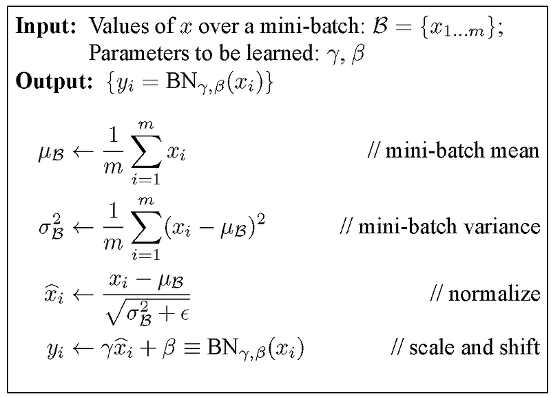
Batch normalization regularizes these gradient from distraction to outliers and flow towards the common goal (by normalizing them) within a range of the mini batch.
Learning rate problem: Generally, learning rates are kept small, such that only a small portion of gradients corrects the weights, the reason is that the gradients for outlier activations should not affect learned activations. By batch normalization, these outlier activations are reduced and hence higher learning rates can be used to accelerate the learning process.
7 — Long Short-Term Memory:
A LSTM network has the following three aspects that differentiate it from an usual neuron in a recurrent neural network:
- It has control on deciding when to let the input enter the neuron.
- It has control on deciding when to remember what was computed in the previous time step.
- It has control on deciding when to let the output pass on to the next time stamp.
The beauty of the LSTM is that it decides all this based on the current input itself. So if you take a look at the following diagram:
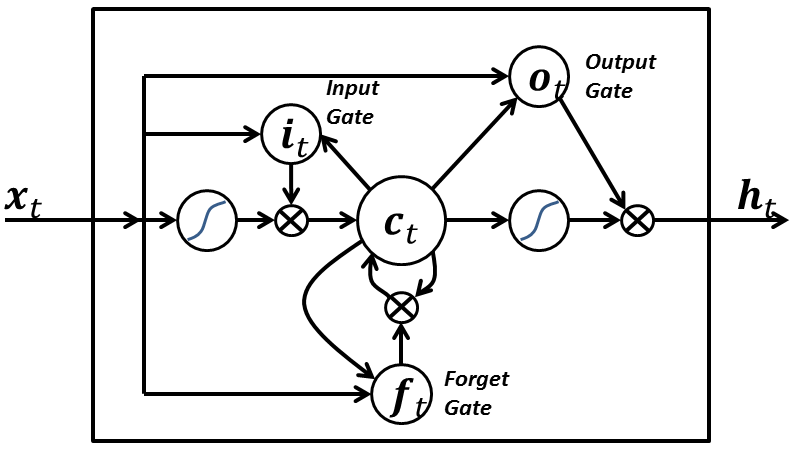
The input signal x(t) at the current time stamp decides all the above 3 points. The input gate takes a decision for point 1. The forget gate takes a decision on point 2 and the output gate takes a decision on point 3. The input alone is capable of taking all these three decisions. This is inspired by how our brains work and can handle sudden context switches based on the input.
8 — Skip-gram:
The goal of word embedding models is to learn a high-dimensional dense representation for each vocabulary term in which the similarity between embedding vectors shows the semantic or syntactic similarity between the corresponding words. Skip-gram is a model for learning word embedding algorithms.
The main idea behind the skip-gram model (and many other word embedding models) is as follows: Two vocabulary terms are similar, if they share similar context.
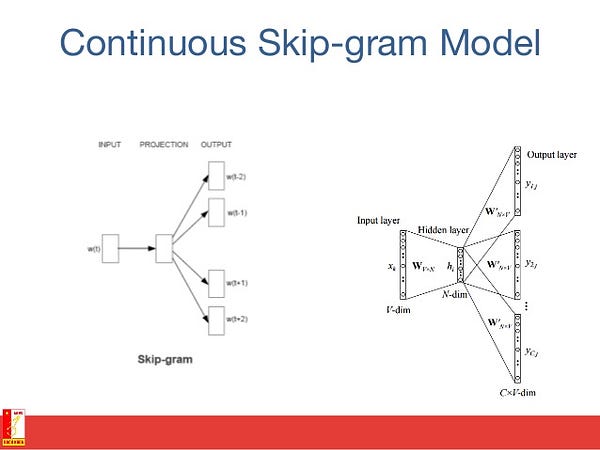
In other words, assume that you have a sentence, like “cats are mammals”. If you use the term “dogs” instead of “cats”, the sentence is still a meaningful sentence. So in this example, “dogs” and “cats” can share the same context (i.e., “are mammals”).
Based on the above hypothesis, you can consider a context window (a window containing k consecutive terms. Then you should skip one of these words and try to learn a neural network that gets all terms except the one skipped and predicts the skipped term. Therefore, if two words repeatedly share similar contexts in a large corpus, the embedding vectors of those terms will have close vectors.
9 — Continuous Bag Of Words:
In natural language processing problems, we want to learn to represent each word in a document as a vector of numbers such that words that appear in similar context have vectors that are close to each other. In continuous bag of words model, the goal is to be able to use the context surrounding a particular word and predict the particular word.
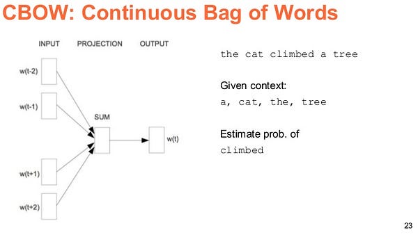
We do this by taking lots and lots of sentences in a large corpus and every time we see a word, we take the surrounding word. Then we input the context words to a neural network and predict the word in the center of this context.
When we have thousands of such context words and the center word, we have one instance of a dataset for the neural network. We train the neural network and finally the encoded hidden layer output represents the embedding for a particular word. It so happens that when we train this over a large number of sentences, words in similar context get similar vectors.
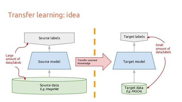
10 — Transfer Learning:
Let’s think about how an image would run through a Convolutional Neural Networks. Say you have an image, you apply convolution to it, and you get combinations of pixels as outputs. Let’s say they’re edges. Now apply convolution again, so now your output is combinations of edges… or lines. Now apply convolution again, so your output is combinations of lines and so on. You can think of it as each layer looking for a specific pattern. The last layer of your neural network tends to get very specialized. Perhaps if you were working on ImageNet, your networks last layer would be looking for children or dogs or airplanes or whatever. A couple layers back you might see the network looking for eyes or ears or mouth or wheels.
Each layer in a deep CNN progressively builds up higher and higher level representations of features. The last couple layers tend to be specialized on whatever data you fed into the model. On the other hand, the early layers are much more generic, there are many simple patterns common among a much larger class of pictures.
Transfer learning is when you take a CNN trained on one dataset, chop off the last layer(s), retrain the models last layer(s) on a different dataset. Intuitively, you’re retraining the model to recognized different higher level features. As a result, training time gets cut down a lot so transfer learning is a helpful tool when you don’t have enough data or if training takes too much resources.
This article only shows the general overview of these methods. I suggest reading the articles below for more detailed explanations:
- Andrew Beam’s “Deep Learning 101”
- Andrey Kurenkov’s “A Brief History of Neural Nets and Deep Learning”
- Adit Deshpande’s “A Beginner’s Guide to Understanding Convolutional Neural Networks”
- Chris Olah’s “Understanding LSTM Networks”
- Algobean’s “Artificial Neural Networks”
- Andrej Karpathy’s “The Unreasonable Effectiveness of Recurrent Neural Networks”
Deep Learning is strongly technique-focused. There are not much concrete explanations for each of the new ideas. Most new ideas came out with experimental results attached to prove that they work. Deep Learning is like playing LEGO. Mastering LEGO is as challenging as any other arts, but getting into it is easier.


