In the last year, graph embeddings have become increasingly important in Enterprise Knowledge Graph (EKG) strategy. Graph embeddings will soon become the de facto way to quickly find similar items in large billion-vertex EKGs. And as we have discussed in our prior articles, real-time similarity calculations are critical to many areas such as recommendation, next best action, and cohort building.
The goal of this article is to give you an intuitive feeling for what graph embeddings are and how they are used so you can decide if these are right for your EKG project. For those of you with a bit of data science background, we will also touch a bit on how they are calculated. For the most part, we will be using storytelling and metaphors to explain these concepts. We hope you can use these stories to explain graph embeddings to your non-technical peers in a fun and memorable way. Let’s start with our first story, which I call “Mowgli’s Walk.”.
Mowgli’s Walk
This story is a bit of fan-fiction based on Rudyard Kipling’s wonderful story, The Jungle Book.

Mowgli is a young boy that lives in a prehistoric village with a sturdy protective wall around it. Mowgli has a cute pet cat with orange fur and stripes. One day, Mowgli walks down a path just outside the village wall and sees a large tiger in the path ahead. What should Mowgli do?
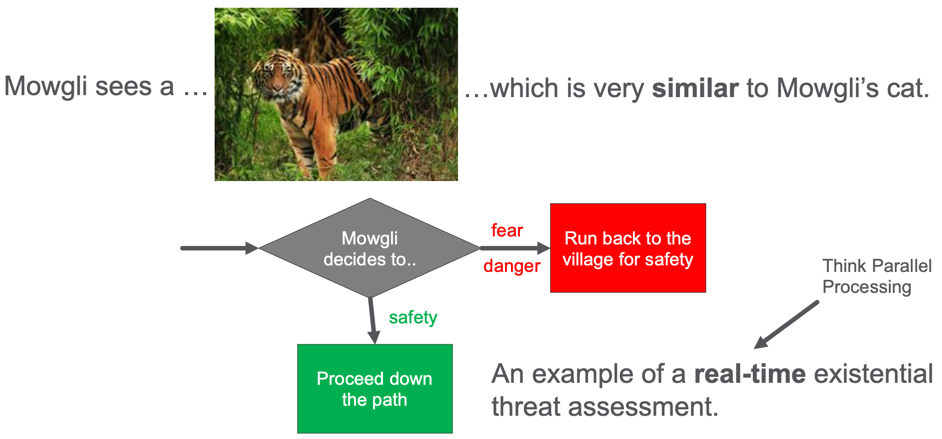
Should he continue down the path or quickly run back to the village and the safety of the wall? Mowgli does not have a lot of time to make this decision. Perhaps only a few seconds. Mowgli’s brain is doing real-time threat detection, and his life depends on a quick decision.
If Mowgli’s brain thinks that the tiger is similar to his pet cat he will proceed down the path. But if he realized that the tiger is a threat, he will quickly run back to the village’s safety.
So let’s look at how Mowgli’s brain has evolved to perform this real-time threat assessment. The image of the tiger arrives through Mowgli’s eyes and is transmitted to his brain’s visual cortex. From there, the key features of the image are extracted. The signals of these features are sent up to the object classification areas of his brain. Mowgli needs to compare this image with every other image he has ever seen and then match it to the familiar concepts. His brain is doing a real-time similarity calculation.
Once Mowgli’s brain matches the image to the tiger concept, and the tiger concept, in turn, is linked to the “danger” emotion, in the fear center of his amygdala, Mowgli will turn around and run back to the village. This fast-response may not even go through the higher-order logic processing in Mowgli’s neocortex. If that had to happen, Mowgli might take additional time to ponder his decision. Mowgli’s genes might get removed from the gene pool. We have evolved data structures in our brain that promote our survival by analyzing millions of inputs from the retina in our eyes to 1/10 of a second.
So now you might be asking, how is this related to graph embeddings? Graph embeddings are small data structures that aid the real-time similarity ranking functions in our EKG. They work just like the classification portions in Mowgli’s brain. The embeddings absorb a great deal of information about each item in our EKG, potentially from millions of data points. Embeddings compress it into data structures that are compact and easy to compare in real-time using low-cost parallel compute hardware like an FPGA. They enable real-time similarity calculations that can be used to classify items in our graph and make real-time recommendations to our users.
For example, a user comes to our e-commerce website looking for a gift for a baby shower. Should we recommend that cute plush tiger toy or a popular new flame thrower? Can we recommend the right item in 1/10th of a second? I believe that in the near future, the ability for a company to quickly respond to customer’s needs and make recommendations on the next best action will be essential for any organization’s survival. We know that EKGs can cost-effectively store tens of thousands of data points about customer history. Embeddings help us analyze this data off-line and use the compressed data in the embedding in real-time.
Now that we know what we want our embedding to do, we can understand why it has a specific structure.
What Are Graph Embeddings?
Before we go into the details of how we store and calculate embeddings, let’s describe the structure of an embedding and the characteristics of what makes embeddings useful for real-time analytics.
- Graph embeddings are data structures used for fast-comparison of similar data structures. Graph embeddings that are too large take more RAM and longer to compute a comparison. Here smaller is often better.
- Graph embeddings compress many complex features and structures of the data around a vertex in our graph including all the attributes of the vertex and the attributes of the edges and vertices around the main vertex. The data around a vertex is called the “context window” which we will discuss later.
- Graph embeddings are calculated using machine learning algorithms. Like other machine learning systems, the more training data we have, the better our embedding will embody the uniqueness of an item.
- The process of creating a new embedding vector is called “encoding” or “encoding a vertex”. The process of regenerating a vertex from the embedding is called “decoding” or generating a vertex. The process of measuring how well an embedding does and finding similar items is called a “loss function”.
- There may not be “semantics” or meaning associated with each number in an embedding. Embeddings can be thought of as a low-dimensional representation of an item in a vector space. Items that are near each other in this embedding space are considered similar to each other in the real world. Embeddings focus on performance, not explainability.
- Embeddings are ideal for “fuzzy” match problems. If you have hundreds or thousands of lines of complex if-then statements to build cohorts, graph embeddings provide a way to make this code much smaller and easier to maintain.
- Graph embeddings work with other graph algorithms. If you are doing clustering or classification, graph embeddings can be used as an additional tool to increase the performance and quality of these other algorithms.
Before we talk about how embeddings are stored, we should review the concept of mathematical nearness functions.
Nearness In Embedding Space
What does it mean for two concepts to be similar? Let’s start with a metaphor of a geographic map.
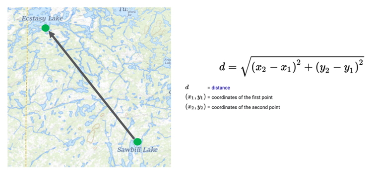
Given two points on the map, we can calculate a distance between these two points by using the distance formula. The inputs are just the coordinates of the two points expressed as numbers such as their longitude and latitude. The problem also can be generalized into three dimensions for two points in space. But in the three-dimensional space version, the distance calculation adds an additional term for the hight or z-axis.
Distance calculations in an embedding work in similar ways. The key is that instead of just two or three dimensions, we may have 200 or 300 dimensions. The only difference is the addition of one distance term for each new dimension.
Word Embedding Analogies
Much of the knowledge we have gained in the graph embeddings movement has come from the world of natural language processing. Data scientists have created precise distance calculations between any two words or phrases in the English language using word embeddings. They have done this by training neural networks on billions of documents and using the probability of a specific word occurring in a sentence when you take all the other words around it into account. Surrounding words become the “context window”. From this, we can effectively do distance calculations on words.
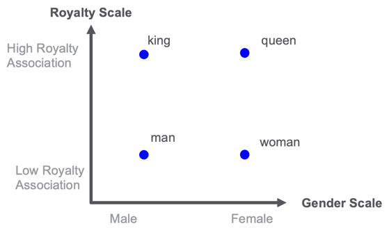
In the example above, imaging putting the words king, queen, man, and woman on a two-dimensional map. One dimension is related to royalty and one dimension is related to gender. Once you have every word scored on these scales you could find similar words. For example, the word “princess” might be closest to the word “queen” in the royalty-gender space.
The challenge here is that manually scoring each word in these dimensions would take a long time. But by using machine learning and having a good error function that knows when a word can be substituted for another word or follows another word this project can be done. We can train a neural network to calculate the embedding for each word. Note that if we have a new word we have never seen before, this approach will not work.
The English language has about 40,000 words that are used in normal speech. We could put each of these words in a knowledge graph and create a pair-wise link between each word and every other word. The weight on the link would be the distance. However, that would be inefficient since by using an embedding, we could quickly recalculate the edge and the weight.
The metaphor is that just like sentences walk between words in a concept graph, we need to randomly walk through our EKG to understand how our customers, products, etc. are related.
How Are Graph Embedding Stored?
A graph embeddings are stored as a vector of numbers that are associated with a vertex or subgraph of our EKG.
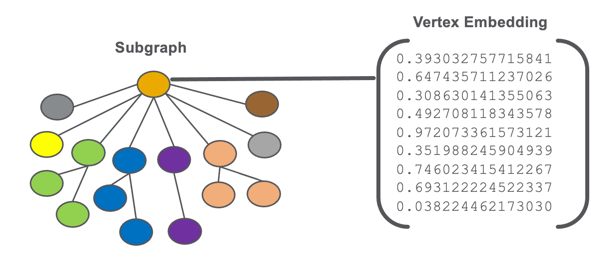
We don’t store strings, codes, dates, or any other types of non-numeric data in an embedding. We use numbers for fast comparison using standardize parallel computation hardware.
Size of Embeddings
Graph embeddings usually have around 100 to 300 numeric values. The individual values are usually 32-bit decimal numbers, but there are situations where you can use smaller or larger data types. The smaller the precision and the smaller the length of the vector, the faster you can compare this item with similar items.
Most comparisons don’t really need more than 300 numbers in an embedding. If the machine learning algorithms are strong, we can compress many aspects of our vertex into these values.
No Semantics with Each Value
The numbers may not represent something that we can directly tie to a single attribute or shape of the graph. We might have a feature called “customer age” but the embedding will not necessarily have a single number for the age feature. The age might be blended into one or more numbers.
Any Vertex Can Have An Embedding
Embeddings can be associated with many things in the EKG. Any important item like a customer, product, store, vendor, shipper, web session, or complaint might have its own embedding vector.
We also usually don’t associate embedding with single attributes. Single attributes don’t usually have enough information to justify the effort of creating an embedding.
There are also projects that are creating embeddings for edges and paths, but they are not nearly as common as a vertex embedding.
Calculating the Context Window of an Embedding
As we mentioned before, the area around a vertex that is used to encode an embedding is called the context window. Unfortunately, there is no simple algorithm for determining the context window. Some embeddings might only look at customer purchases from the last year to calculate an embedding. Other algorithms might look at lifetime purchases and searches that go back since the customer first visited a web site. Understanding the impact of time on an embedding, called temporal analysis, is something that might require additional rules and tuning. Clearly, a customer that purchased baby diapers on your web site 20 years ago might be very different than someone that just started purchasing them last month.
Embeddings vs. Hand-coded Feature Engineering
For those of you that are familiar with standard graph similarity algorithms such as cosine similarity calculations, we want to do a quick comparison. Cosine similarity also creates a vector of features which are also simple numeric values. The key difference is that manually creating these features takes time and the feature engineer needs to use their judgment on how to scale the values so the weights are relevant. Both age and gender might have a high weight and a feature that scores a person’s preference for chocolate or vanilla ice cream might not be relevant for general-purpose item purchases.
Embeddings try to use machine learning to automatically figure out what features are relevant for making predictions about an item.
Tradeoffs of Creating Embeddings
When we design EKGs, we work hard to not load data into RAM that does not provide value. But embeddings do take up valuable RAM. So we don’t want to go crazy and create embeddings for things that we rarely compare. We want to focus on when similarity calculations get in the way of real-time responses for our users.
Homogeneous vs. Heterogeneous Graphs
Many early research papers on graph embedding focused on simple graphs where every vertex has the same type. These are called homogeneous or monopartite graphs. One of the most common examples is the citation graph where every vertex is a research paper and all the links are to other research papers that are cited by a paper. Social networks where every vertex is a person and the only link type is “follows” or “friend-of” is another type of homogeneous graph. Word embeddings, where every word or phrase has an embedding, is another example of a homogeneous graph.
Unfortunately, knowledge graphs usually have many different types of vertices and many types of edges. These are known as multipartite graphs. And they make the process of calculating embeddings more complicated. A customer graph may have types such as Customer, Product, Purchase, Web Visit, Web Search, Product Review, Product Return, Product Complaint, Promotion Response, Coupon Use, Survey Response, etc. Creating embeddings from complex data sets can take time to set up and tune the machine learning algorithms.
How Enterprise Knowledge Graph Embeddings Are Calculated
For this article, we are going to assume you have a large EKG. By definition, an EKG does not fit in the RAM of a single server node and must be distributed over tens or hundreds of servers. This means that simple techniques like creating an adjacency matrix are out of the question. We need algorithms that scale and work on distributed graph clusters.
There are around 1,400 papers on Google Scholer that mention the topic of “knowledge graph embeddings”. I don’t claim to be an expert on all the various algorithms. In general, they fall into two categories.
- Graph convolutional neural networks (GCN)
- Random walks
Let’s briefly describe these two approaches before we conclude our post.
Graph Convolutional Neural Networks (GCN)
The GCN algorithms take a page from all the work that has been done with convolutional neural networks in image processing. Those algorithms look at the pixels around a given pixel to come up with the next layer in the network. Images are called “Euclidean” spaces since the distance between the pixels is uniform and predictable. GCNs use roughly the same approach by looking around a current vertex, but the conceptual distances are non-uniform and unpredictable.
Random Walk Algorithms
These algorithms tend to follow the research done in natural language processing. They work by randomly traversing all the nodes starting from a target node. The walks effectively form sentences about the target vertex and these sequences are then used the same way that NLP algorithms work.
Conclusion
I hope that the stories and metaphors in this blog post give you a better intuitive feel for what graph embeddings are and how they are used to accelerate real-time analytics. Although you might be discouraged by the fact that there is no definitive library of functions for calculating embeddings on all platforms, I think you will see from the amount of research being published that this is an active area of research. I think that just like AlexNet broke ground in image classification and BERT set a new standard for NLP, that within the next few years we will see graph embedding take center stage in the area of innovative analytics.
Note: For anyone that is attending the virtual Neural Information Processing Systems (NeurIPS 2020) conference this year, there are 114 events related to embedding. Embeddings are clearly a hot topic in deep learning.


