Summations, factorials, matrices and more are simple when we look at them with our favorite languages
Summations, factorials, matrices and more are simple when we look at them with our favorite languages

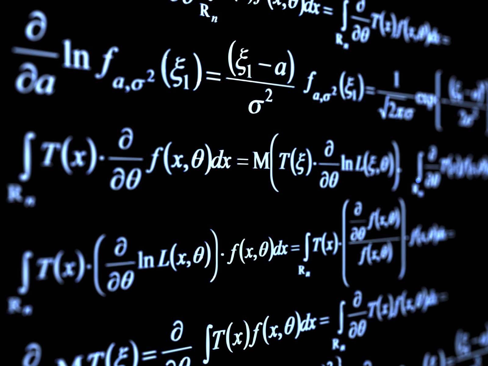
For anyone interested in pursuing a career or research in Machine Learning and Data Science, the day will come when it is time to move beyond the python libraries to follow curiosities into the math behind it all. This will typically take you to the vast, open collection of papers detailing how it all works. The deeper you go to understand the core mathematics, the closer you may come to the flash of insight to create a new method. Everything seems to be all right on the first paper until you come across something like this:

For anyone who has studied math for years or worked at the math level of Machine Learning, such an equation can be carefully parsed into meaning and code. For many others though, this may look like hieroglyphics. The truth is that it almost seems like the ancient math leaders chose the most interesting looking symbols to describe rather intuitive methods. The result: Equations and variables that look much more complex than they really are.
I’ve found that code can be used for more than writing programs, but also a globally agreed-upon language to explain the complex. When I was learning the math behind everything Data Science, I always found that the best way to gain a universal understanding of math was to write code snippets to describe equations. Eventually, these symbols become understood to a point that they can almost be read as text in a typical paper. In this article, I hope to share some examples of how simple math can be when described with code!
Summation and Product

The summation symbol is one of the most useful and commonly used symbols in iterative mathematics. Despite its complex design, the implementation is rather simple, yet incredibly useful.
As seen above, all that this symbol represents is a for loop in the range of the number on top, starting from the number on the bottom. The variable set on the bottom becomes the index variable and any result per loop is added to an overall value. Less commonly, the following may be used:
![]()
Typically called the Product Operator, this symbol functions in the same manner, but instead of adding each result they will be multiplied.
Factorial
Factorial is the “!” which exists on almost any calculator. To many, this one may be a bit more obvious, but it is still worth it to write some code to understand the mechanics.
5! would be represented as:
Conditional Brackets
Conditional brackets are used to divert the flow of an equation based on a set of conditions. For coders, this is simply the common “if” statement. The above conditional can be represented as:
As seen above, the right notation of each row of the bracket dictates what each path should execute. I threw the extra “contains” symbol into each condition as well to add more insight. As seen above, we checked if the i value was in the y list. Recognizing that it was, we returned the sum of the array. If the i value had not been in the array we would have returned 0 or 1 based on the value.
Point Wise and Cartesian Matrix Multiplication
Finally, I wanted to quickly cover the operations which are typically done for any Data Scientist by their favorite language library — matrix multiplication. The easiest form to understand is the point wise operation. This is simply written as:

Note the first requirement is that each matrix must have the same shape(ie # rows= & #Columns=)
The code for this looks as follows:
Lastly let’s take a look at a typical matrix multiplication process, most commonly used in Machine Learning. In complex terms, this operation finds the dot product of each primary row with each secondary column. The main take away from this is the the following requirement: assume [#rows, #columns] →matrices i x j requires #columns(i) == #rows(j) → with a final product of shape [#rows(i), #columns(j)]
This may seem confusing and my best suggestion would be to take a look at google images for some great visualizations of these requirements.

The code for this equation looks as follows(using numpy dot method):
This was just a few examples, but the understanding of this simple code can allow any programmer to take on the initially ominous world of mathematics. Of course, these methods can all be consolidated for efficiency and usually have a library method readily available. The point of writing these in simple code is to see how much sense they make when written out in the form of their true operations.


