What is Probabilistic Programming?
The idea behind Probabilistic programming to bring the inference algorithms and theory from statistics combined with formal semantics, compilers, and other tools from programming languages to build efficient inference evaluators for models and applications from Machine Learning. In other words, probabilistic programming is a tool for statistical modeling. The idea is to borrow lessons from the world of programming languages and apply them to the problems of designing and using statistical models.
Probabilistic programming is about doing statistics using the tools of computer science.
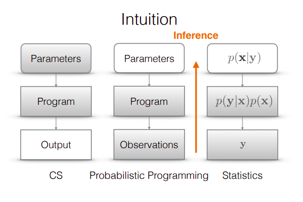
In the above figure you can see a typical computer science programming pipeline: Write a program, specify the values of its arguments then evaluate the program to produce an output. The right-hand side illustrates the approach taken to modeling in statistics: Start with the output, the observations or data Y, then specify an abstract generative model p(X,Y), often denoted mathematically, and finally use algebra and inference techniques to characterize the posterior distribution, p(X | Y ), of the unknown quantities in the model given the observed quantities. Whereas in Probabilistic programming: a programming language for model definitions and statistical inference algorithms for computing the conditional distribution of the program inputs that could have given rise to the observed program output.
Note: Probabilistic programming is not about writing software that behaves probabilistically.
To implement such Ensemble Architecture Tensorflow introduces Tensorflow-probability.
Tensorflow-Probability
TensorFlow Probability is a library for probabilistic reasoning and statistical analysis in TensorFlow. As part of the TensorFlow ecosystem, TensorFlow Probability provides integration of probabilistic methods with deep networks, gradient-based inference via automatic differentiation, and scalability to large datasets and models via hardware acceleration (e.g., GPUs) and distributed computation.
Probabilistic Machine Learning tools in TensorFlow-probability are structured in different levels. In this blog, we’ll discuss Statistical building blocks and Model Building using TensorFlow-probability.
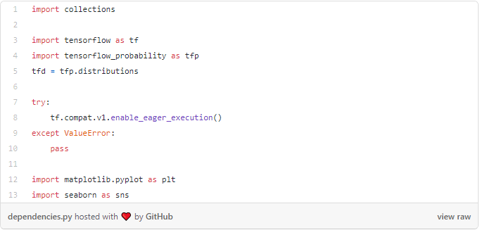
Let’s start with importing necessary modules:
Statistical Functions in Tensorflow-probability
Distributions-
A tfp.distributions.Distribution is a class with two core methods: sample and log_prob. This class contains many distributions which can be seen by writing:
print_subclasses_from_module(tfp.distributions, tfp.distributions.Distribution)
Let’s see how to sample a Normal Distribution which is a good starter in stat101 using tf-probability:
# A standard normal
normal = tfd.Normal(loc=0., scale=1.) # mean=0, std=3samples = normal.sample(1000)
sns.distplot(samples)
plt.title("Samples from a standard Normal")
plt.show()'''
log of the probability density/mass function evaluated at the given sample value.
'''
print("log(PDF):",normal.log_prob(0.))
Now in order to calculate other statistical parameters like cumulative distribution function and multiple distributions we can still utilize tf-probabilities native classes.
# Define a single scalar Normal distribution.
dist = tfd.Normal(loc=0., scale=3.)  # mean=0, std=3# Evaluate the cdf at 1, returning a scalar.
dist.cdf(1.)# Define a batch of two scalar valued Normals.
# The first has mean 1 and standard deviation 11, the second 2 and 22.
dist = tfd.Normal(loc=[1, 2.], scale=[11, 22.])# Evaluate the pdf of the first distribution on 0, and the second on 1.5,
# returning a length two tensor.
dist.prob([0, 1.5])# Get 3 samples, returning a 3 x 2 tensor.
dist.sample([3])
Using the above code you can calculate CDFs and Multiple Normal Distributions on-the-fly.
While using statistical-tools in your project you might also require declaring Multivariate Distributions, tf-probability has got you covered here as well!
mvn = tfd.MultivariateNormalDiag(loc=[0., 0.], scale_diag = [1., 1.])
print("Batch shape:", mvn.batch_shape)
print("Event shape:", mvn.event_shape)samples = mvn.sample(1000)
print("Samples shape:", samples.shape)g = sns.jointplot(samples[:, 0], samples[:, 1], kind='scatter')
plt.show()
There are tons of distributions like these inside the tfp module, LogNormal, Logistic, LogitNormal Mixture, Multinomial, MultivariateNormalDiag, to name a few. Every distribution comes with a plethora of statistical inferences and functions.
Bijectors-
Bijectors represent invertible, smooth functions. They can be used to transform distributions, preserving the ability to take samples and compute log_probs. They can be accessed from the tfp.bijectors module.
Each bijector implements at least 3 methods:
forwardinverse, and- (at least) one of
forward_log_det_jacobianandinverse_log_det_jacobian.
With these ingredients, we can transform a distribution and still get samples and log probs from the result!
print_subclasses_from_module(tfp.bijectors, tfp.bijectors.Bijector)
Using the code snippet above we can list all the bijector functions available in tf-probability.
Now let’s see how to declare a NormalCDF using bijectors and calculate the log of the determinant of the Jacobian in forward propagation.
normal_cdf = tfp.bijectors.NormalCDF()
xs = np.linspace(-4., 4., 200)
plt.plot(xs, normal_cdf.forward(xs))
plt.show()plt.plot(xs, normal_cdf.forward_log_det_jacobian(xs, event_ndims=0))
plt.show()
Bijectors are mainly used for transforming Distributions. Here’s a quick example where transformation is applied:
# creates a Y=g(X)=exp(X) transform
exp_bijector = tfp.bijectors.Exp()# declare a Normal Distribution and Transform it
log_normal = exp_bijector(tfd.Normal(0., .5))

samples = log_normal.sample(1000)
xs = np.linspace(1e-10, np.max(samples), 200)sns.distplot(samples, norm_hist=True, kde=False)
plt.plot(xs, log_normal.prob(xs), c='k', alpha=.75)
plt.show()
After running the above snippet you’ll see a transformed distribution(bins in blue) and probability density estimation plot (curve in black)
We successfully implemented the building blocks of statistical inference in Tensorflow-probability, now let’s see how we can use the same framework with tabular time-series data.
Timeseries with Tensorflow-Probability
TensorFlow-Probability (TFP) features built-in support for fitting and forecasting using structural time series models. This support includes the Bayesian inference of the model. Because they’re built-in TensorFlow, these methods naturally take advantage of vectorized hardware (GPUs and TPUs), can efficiently process many time series in parallel, and can be integrated with deep neural networks.
Let’s solve a time-series problem using TensorFlow-probability:
Importing necessary modules:
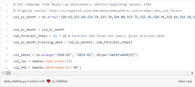
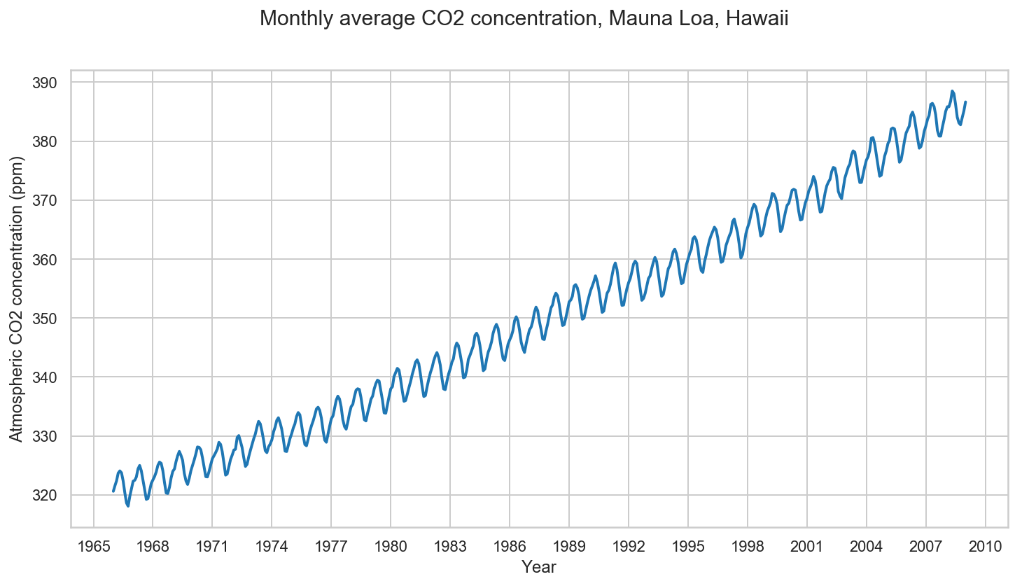
Now let’s define a time-series problem of Co2 concentration over the years (sampled by month):
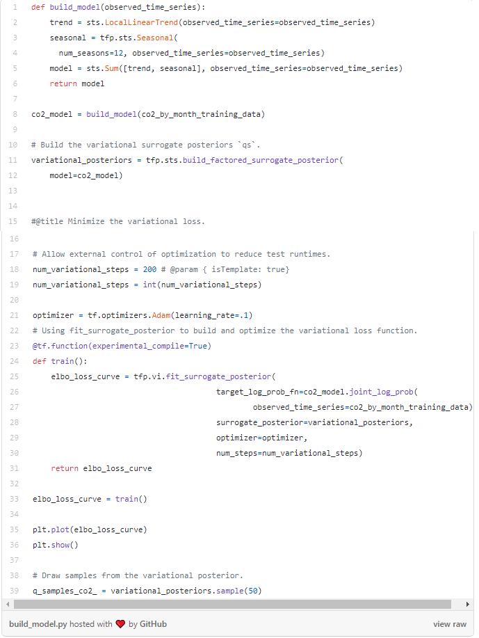
Model and Fitting
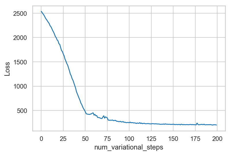
We’ll model this series with a local linear trend, plus a month-of-year seasonal effect, and fit the model using variational inference. This involves running an optimizer to minimize a variational loss function, the negative evidence lower bound (ELBO). This fits a set of approximate posterior distributions for the parameters (in practice we assume these to be independent Normals transformed to the support space of each parameter).
The tfp.sts forecasting methods require posterior samples as inputs, so we’ll finish by drawing a set of samples from the variational posterior.
After running the above script you’ll see a plot like this:
Forecasting
Now let’s use the fitted model to construct a forecast. We just call tfp.sts.forecast, which returns a TensorFlow Distribution instance representing the predictive distribution over future timesteps.
In particular, the mean and stddev of the forecast distribution give us a prediction with marginal uncertainty at each timestep, and we can also draw samples of possible futures.
Lets now visualize the forecast of the Co2 Concentration.
We can observe here that the forecast made by our model turned out pretty good. It was able to capture seasonal changes and the overall trend of the time-series and able to predict the Co2 concentrations as it happened.
Let’s now see the Trend and Seasonality of the Co2 concentration:
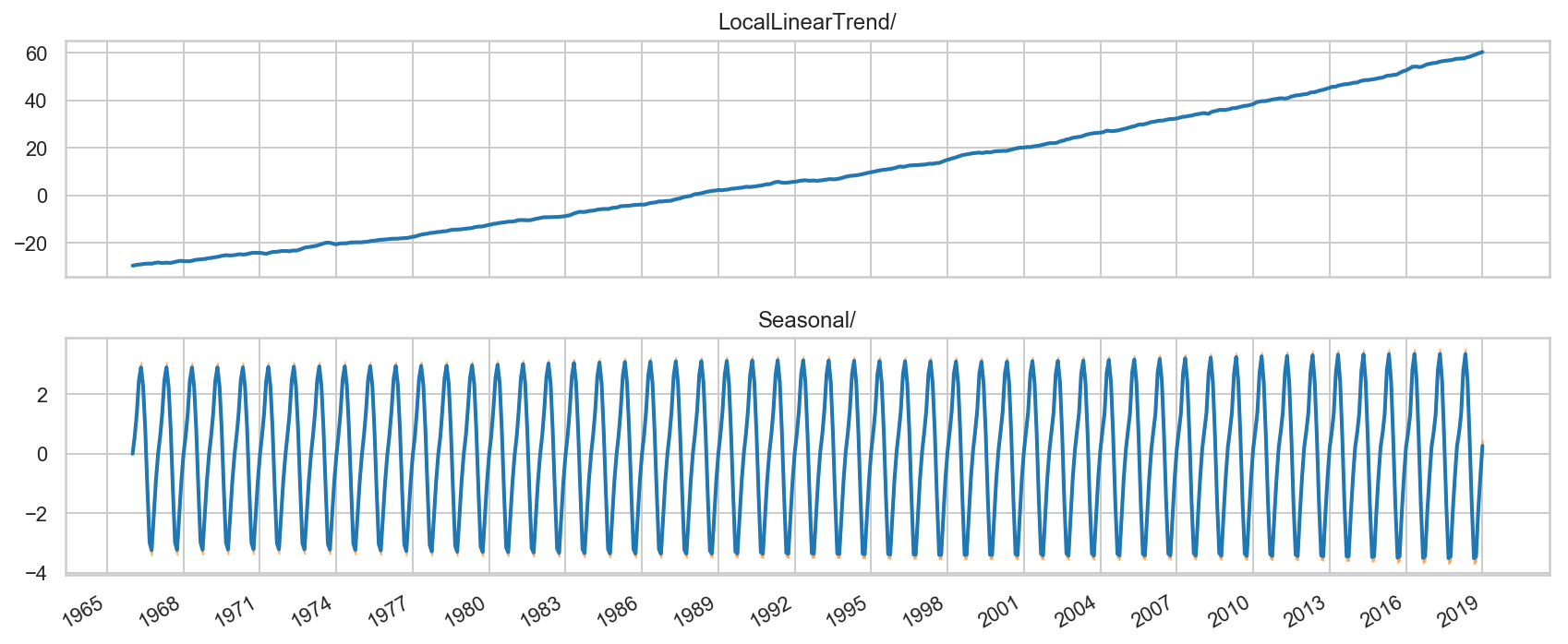
As we already discussed how statistical inferences and tools can be easily implemented through TFP. In the above plot, we can identify trends and seasonality from the data just as efficiently as other core stats modules.
You’ve reached the end!
Congratulations! we just learned about the use and importance of Probabilistic-programming and discussed statistical tools in TensorFlow-probability. Not to mention we just solved a structured time-series problem using models from Tensorflow-probability!