Decision Trees are great and are useful for a variety of tasks. They form the backbone of most of the best performing models in the industry like XGboost and Lightgbm.
But how do they work exactly? In fact, this is one of the most asked questions in ML/DS interviews.
We generally know they work in a stepwise manner and have a tree structure where we split a node using some feature on some criterion.
But how do these features get selected and how a particular threshold or value gets chosen for a feature?
In this post, I will talk about three of the main splitting criteria used in Decision trees and why they work. This is something that has been written about repeatedly but never really well enough.
1. Gini Impurity
According to Wikipedia,
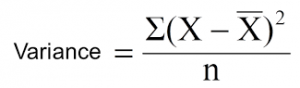
Gini impurity is a measure of how often a randomly chosen element from the set would be incorrectly labeled if it was randomly labeled according to the distribution of labels in the subset.In simple terms, Gini impurity is the measure of impurity in a node. Its formula is:

where J is the number of classes present in the node and p is the distribution of the class in the node.
So to understand the formula a little better, let us talk specifically about the binary case where we have nodes with only two classes.
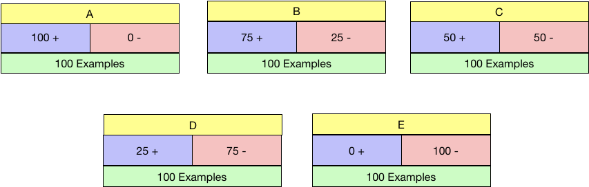
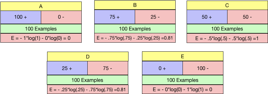
So in the below five examples of candidate nodes labelled A-E and with the distribution of positive and negative class shown, which is the ideal condition to be in?
I reckon you would say A or E and you are right. What is the worst situation to be in? C, I suppose as the data is precisely 50:50 in that node.
Now, this all looks good, intuitively. Gini Impurity gives us a way to quantify it.
Let us calculate the Gini impurity for all five nodes separately and check the values.
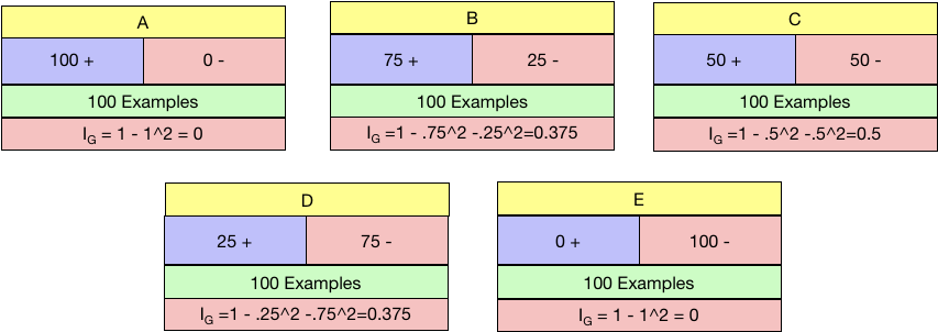
Gini Impurity works as expected. Maximum for Node C and the minimum for both A and E. We need to choose the node with Minimum Gini Impurity.
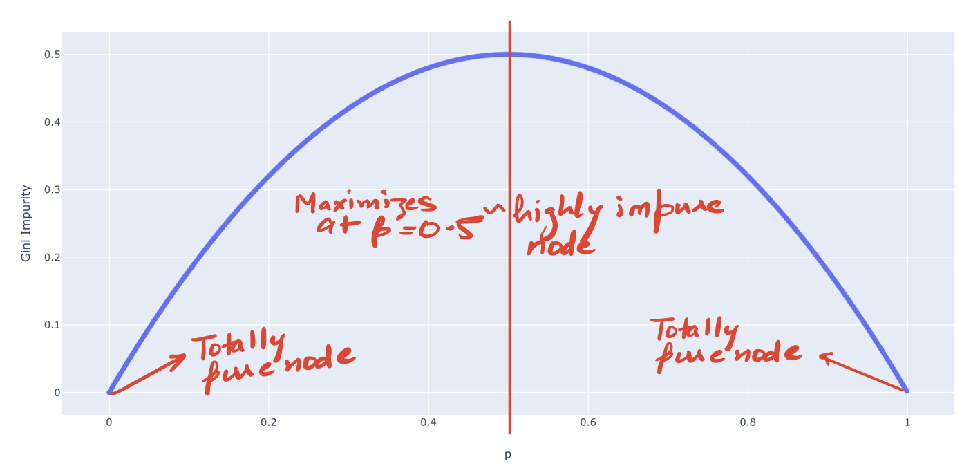
We could also see the plot of Gini Impurity for the binary case to verify the above.
So how do we exactly use it in a Decision Tree?
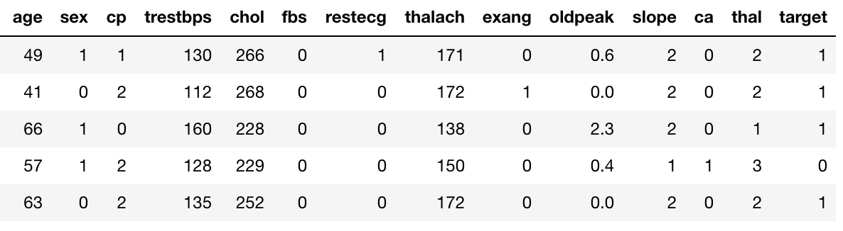
Suppose, we have the UCI Heart Disease data. The “target” field refers to the presence of heart disease in the patient. It is 0 (no presence) or 1.
We now already have a measure in place(Gini Impurity) using which we can evaluate a split on a particular variable with a certain threshold(continuous) or value(categorical).
Categorical Variable Splits
For simplicity, let us start with a categorical variable — sex.
If we split by Sex, our tree will look like below:
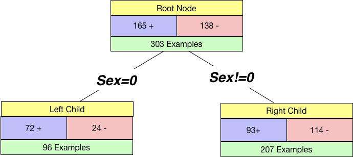
Notice that we use Sex=0 and Sex!=0 so that this generalises well to categories with multiple levels. Our root node has 165 +ve examples and 138 -ve examples. And we get two child nodes when we split by sex.
We already know how to calculate the impurity for a node. So we calculate the impurity of the left child as well as the right child.
I_Left = 1 - (72/96)**2 - (24/96)**2
I_Right = 1 - (93/207)**2 - (114/207)**2

print("Left Node Impurity:",I_Left)
print("Right Node Impurity:",I_Right)
Left Node Impurity: 0.375
Right Node Impurity: 0.4948540222642302
We get two numbers here. We need to get a single number which provides the impurity of a single split. So what do we do? Should, we take an average? We can take an average, but what will happen if one node gets only one example and another node has all other examples?
To mitigate the above, we take a weighted average of the two impurities weighted by the number of examples in the individual node. In code:
gender_split_impurity = 96/(96+207)*I_Left + 207/(96+207)*I_Right
print(gender_split_impurity)
0.45688047065576126
Continuous Variable Splits
We can split by a continuous variable too. Let us try to split using cholesterol feature in the dataset. We chose a threshold of 250 and created a tree.
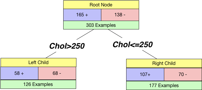
I_Left = 1 - (58/126)**2 - (68/126)**2
I_Right = 1 - (107/177)**2 - (70/177)**2

print("Left Node Impurity:",I_Left)
print("Right Node Impurity:",I_Right)
Left Node Impurity: 0.49685059208868737
Right Node Impurity: 0.47815123368125373
Just by looking at both the impurities close to 0.5, we can infer that it is not a good split. Still, we calculate our weighted Gini impurity as before:
chol_split_impurity = 126/(126+177)*I_Left + 177/(126+177)*I_Right
print(chol_split_impurity)
0.48592720450414695
Since the chol_split_impurity>gender_split_impurity, we split based on Gender.
In reality, we evaluate a lot of different splits. With different threshold values for a continuous variable. And all the levels for categorical variables. And then choose the split which provides us with the lowest weighted impurity in the child nodes.
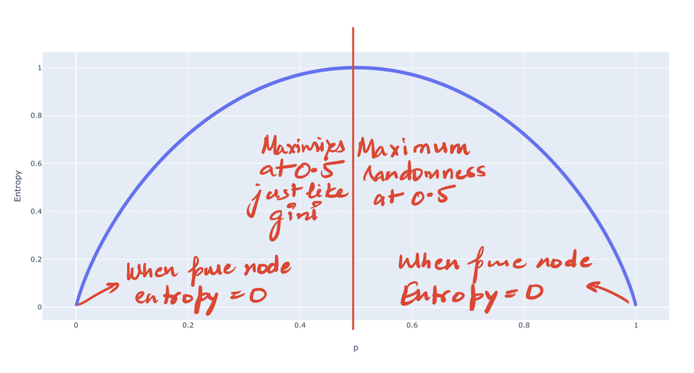
2. Entropy

Another very popular way to split nodes in the decision tree is Entropy. Entropy is the measure of Randomness in the system. The formula for Entropy is:
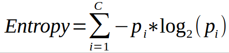
where C is the number of classes present in the node and p is the distribution of the class in the node.
So again talking about the binary case we talked about before. What is the value of Entropy for all the 5 cases from A-E?
Entropy values work as expected. Maximum for Node C and the minimum for both A and E. We need to choose the node with Minimum Entropy.
We could also see the plot of Entropy for the binary case to verify the above.
So how do we exactly use Entropy in a Decision Tree?
We are using the Heartrate example as before. We now already have a measure in place(Entropy) using which we can evaluate a split on an individual variable with a certain threshold(continuous) or value(categorical).
Categorical Variable Splits
For simplicity, let us start with a categorical variable — sex.
If we split by Sex, our tree will look like below:
If we split on Gender
We already know how to calculate the randomness for a node. So we calculate the randomness of the left child as well as the right child.
E_Left = -(72/96)*np.log2(72/96) - (24/96)*np.log2(24/96)
E_Right = -(93/207)*np.log2(93/207) - (114/207)*np.log2(114/207)

print("Left Node Randomness:",E_Left)
print("Right Node Randomness:",E_Right)
Left Node Randomness: 0.8112781244591328
Right Node Randomness: 0.992563136012236
We get two numbers here. We need to get a single number which provides the Randomness of a single split. So what do we do? We again take a weighted average where we weight by the number of examples in the individual node. In code:
gender_split_randomness = 96/(96+207)*E_Left + 207/(96+207)*E_Right
print(gender_split_randomness)
0.9351263006686785
Continuous Variable Splits
Again as before, we can split by a continuous variable too. Let us try to split using cholesterol feature in the dataset. We chose a threshold of 250 and create a tree.
E_Left = -(58/126)*np.log2(58/126) - (68/126)*np.log2(68/126)
E_Right = -(107/177)*np.log2(107/177) - (70/177)*np.log2(70/177)

print("Left Node Randomness:",E_Left)
print("Right Node Randomness:",E_Right)
Left Node Randomness: 0.9954515828457715
Right Node Randomness: 0.9682452182690404
Just by looking at both the randomness close to 1, we can infer that it is not a good split. Still, we calculate our weighted Entropy as before:
chol_split_randomness = 126/(126+177)*E_Left + 177/(126+177)*E_Right
print(chol_split_randomness)
0.9795587560138196
Since the chol_split_randomness>gender_split_randomness, we split based on Gender. Precisely the same results we got from Gini.
3. Variance
Gini Impurity and Entropy work pretty well for the classification scenario.
But what about regression?
In the case of regression, the most common split measure used is just the weighted variance of the nodes. It makes sense too: We want minimum variation in the nodes after the split.
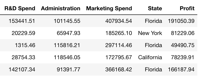
We want a regression task for this. So, we have the data for 50 startups, and we want to predict Profit.
Categorical Variable Splits
Let us try a split by a categorical variable ⇒State=Florida.
If we split by State=FL, our tree will look like below:
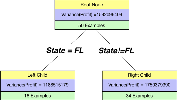
Overall Variance then is just the weighted sums of individual variances:
overall_variance = 16/(16+34)*Var_Left + 34/(16+34)*Var_Right
print(overall_variance)
1570582843
Continuous Variable Splits
Again as before, we can split by a continuous variable too. Let us try to split using R&D spend feature in the dataset. We chose a threshold of 100000 and create a tree.
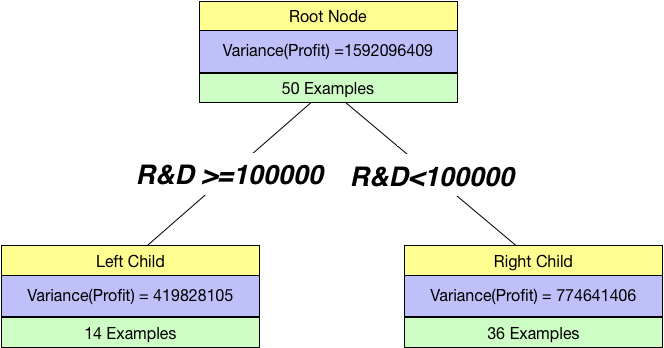
Splitting on R&D
Just by looking at this, we can see it is better than our previous split. So, we find the overall variance in this case:overall_variance = 14/(14+36)*419828105 + 36/(14+36)*774641406
print(overall_variance)675293681.7199999
Since the overall_variance(R&D>=100000)< overall_variance(State==FL), we prefer a split based on R&D.