I’ve recently stumbled upon a Microsoft Azure tool called Microsoft Azure Machine Learning Studio, which is a graphical, web interface to perform machine learning operations using a visual workflow, without the need of writing any code.
I’ve always been a coder and R has been my professional partner since the University period, so I’ve always had little confidence in graphical software. When I discovered ML Studio and performed in a few hours what could reasonably take a few days of coding in R, I’ve definitely added ML Studio to my Data Science Toolbox.
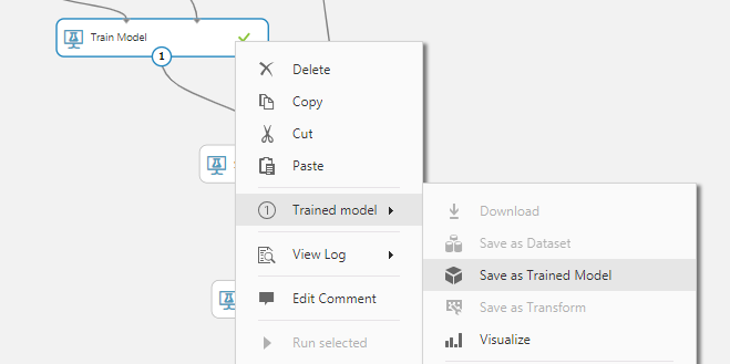
Right-clicking the training node and selecting “Run” will train our model on the training dataset.
The steps I’ll follow are the following:
- Data import
- Basic data analysis
- Training/test split
- Data normalization
- Model selection with cross-validation
- Training of the best model
- Scoring on the holdout dataset
- Evaluation of the performance
Free subscription
At the day I’m writing this article, Azure ML Studio comes with a free subscription and many paid subscriptions based on API usage or disk storage. The free subscription comes with 10 GB of disk space and is enough for educational purposes or small-sized experiments. By the way, “Experiment” is the name that ML studio uses to identify a visual workflow. It’s not the only thing we can do with this software since it comes with the well known Jupyter notebooks as well. However, in this article, I’ll cover only the visual part of ML studio, i.e. the experiments.
In order to create a free subscription, you can visit the URL https://azure.microsoft.com/en-us/services/machine-learning-studio/, click the “Get started now” button and then select the “Free worskspace” plan. If you already have a Microsoft account (for example, if you have ever used Skype), you can attach an ML Studio subscription to this account; otherwise, you’ll need to create one.
First approach
After you’ve finished the subscription procedure, the first window you’ll see opening ML Studio is the following:
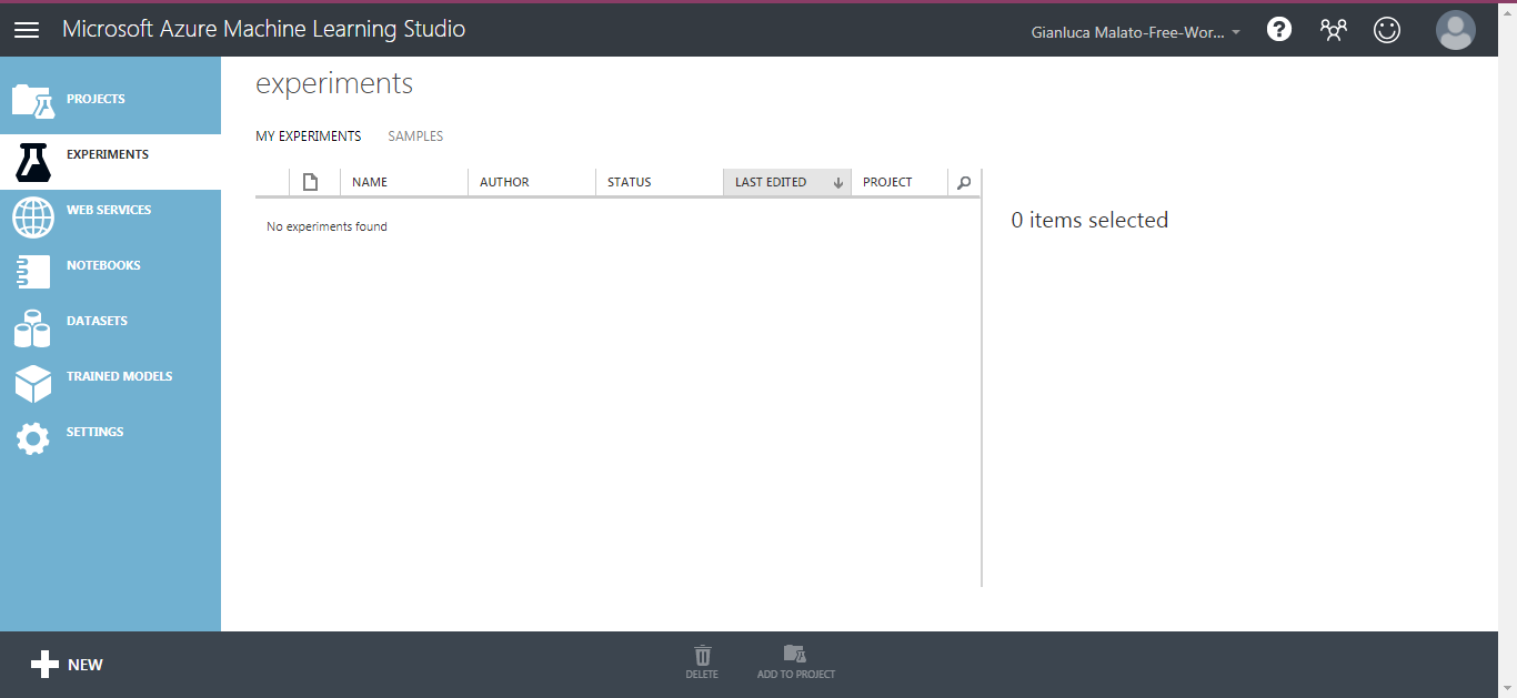
On the left sidebar, we can find many useful features of ML studio, but in this article, I’ll cover only the experiments part.
Clicking on the “Experiments” button and then on the “New” button, we can then create a “Blank experiment” or load a pre-defined one from the gallery.
The main screen we are going to work with most of the time is the following:

The left column contains all the controls that can be dragged and dropped in the central part. The right sidebar is related to the parameters and options of the nodes.
Now, we can start with the interesting stuff.
Data import
ML studio can handle data coming from different sources. It’s possible to upload a dataset from a flat file or reading it from an Azure SQL Database, an URL or even a blob in an Azure Storage Account. The only thing you have to keep in mind is that ML studio supports only a limited number of formats, including CSV and TSV (tab separated values). Concerning the separator, you have only a few fixed options among which you can choose, so be careful when you create a dataset; first, make sure you use a format that ML Studio recognizes.
For this simple example, I’ll use the famous Iris dataset. ML Studio contains many example datasets, including a modified version of the Iris dataset, suitable for a binary classification problem.
If you go to “Saved Datasets” and then on “Samples”, you’ll find all the available example sets.

Search for “Iris two class data” and drag it on the central part of the screen.

The circle with the number 1 in the bottom side of the node is an output port. In ML Studio, each node can have several input and output ports, identified by circles and number. The input ports are located on the upper side of the node and specify the input data the node has to manipulate. The output ports are located at the bottom and are used to distribute the output of the node as an input to other nodes. Connecting the nodes through their ports makes us design a complete workflow.
Datasets don’t have input port because they don’t crunch data of any kind (they only deliver it).
Basic data analysis
Before manipulating this dataset in any way, we can take a look at it. Let’s right-click the node and select “Dataset”, then “Visualize”.

This is the window that appears:
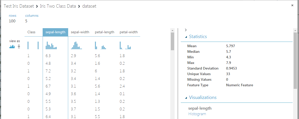
The central part contains a sample of the dataset and some thumbnails of the histograms of each column, that can be selected individually.
The right part contains some basic statistics about the column you select.
If you scroll down, you’ll see a histogram of the selected variable.

A useful feature is a possibility to plot one variable against another one via the “Compare to” dropdown menu.

As you can see, this plot highlights a strong, visual correlation between the sepal length and the class variables. It’s a very useful piece of information about the importance of this feature.
Training/test split
The next thing we have to do with our dataset is deciding which part of it we want to use as the training dataset. The remaining part will be used as a test dataset (sometimes called holdout), which will be used only for the final model evaluation.
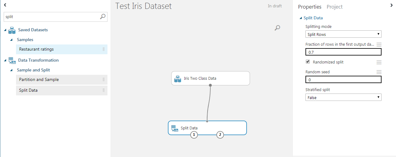
We can use the “Split Data” node and connect its input to the output of the dataset.
This way, we are telling ML studio “Use the output of iris dataset node as an input to the split node”.
On the right part, you can see the options of the node. We can use a 0.7 ratio for the training dataset, while the remaining 0.3 is used for the test set. The split is performed randomly.
The two output ports of the split node are, respectively, the training dataset (port number 1) and the test dataset (port number 2).
Data normalization
In machine learning, it’s frequent that data must be prepared for our model in a proper way. The reasons are many and depend on model nature. Logistic regression and neural networks work quite well when the input variables are scaled between 0 and 1. That’s due to the fact that logistic function saturates easily for input values that are greater than 2 on absolute value, so their importance could be misunderstood by the model. With a 0-1 scaling, the minimum value of each variable becomes 0 and the maximum value becomes 1. The other values are scaled proportionally. Don’t forget that scaling of the features is an important part of the pre-processing part of a machine learning pipeline.
So, we need to use the “Normalize Data” node. From the options panel, we can choose MinMax (that is, 0–1 range).
The input of the Normalize Data node is the training dataset, so we connect it to the first output port of the split data node.

The Normalize Data node has two output ports. The first one is the scaled input dataset, the second one make possible to use the scaling transformation in other datasets. It will soon be useful.
Model selection with cross-validation
Now we have prepared our data for the training phase. We are working with a binary classification problem and, in this example, we’ll work with logistic regression and a neural network, choosing the best one among the two models.
For each one of the two models, we’ll perform k-fold cross-validation in order to check their average performance on unseen data and then select the model that has the highest performances.
Let’s start adding the Logistic Regression node by searching for the word “logistic”.

We can select the node “Two-Class Logistic Regression” and drag it into the workspace.
Then we can search “cross” and will find the “Cross Validate Model” node.

We can connect the nodes as shown in the next figure:

On the right part, we must select the target variable:

Click on “Launch column selector” and select the “Class” variable, as shown in the next picture.

Now we can run the cross-validation process by right-clicking the “Cross Validate Model” node and selecting “Run selected”.

After the process has ended, we can right click again and select “Evaluation results by fold”, then “Visualize”.

The following picture shows the evaluation performance metric for each one of the 10 default folds for cross-validation. We’ll check the Area under the ROC curve (often called AUC) as a metric to compare different models. The higher this value, the better the model.
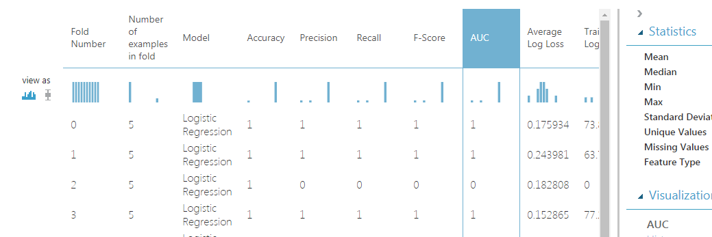
Scrolling down we’ll reach the “Mean” row, which contains the mean values of the performance metrics calculated among the folds.

The mean value of Logistic Regression’s AUC is 0.9. Let’s keep it in mind.
Now it’s time for the neural network, so we’ll repeat the process and search for the word “neural” in the search box.

We need the “Two-Class neural network” node, so let’s drag it together with the cross-validation node as the following picture.

Neural networks have many hyperparameters, so we must choose at least how many neurons we want to use in the hidden layer. For this example, we’ll select 5 hidden nodes.
Click on the “Two-Class Neural Network” node and change the “Number of hidden nodes” to 5.

As you can see, it’s equal to the logistic regression performance. It’s due to the nature of iris dataset, which is chosen to make every model work properly.
If one of the two models would have reached higher performances than the other one, we would have selected it. Since the performances are the same and we want the simplest model possible, we’ll choose the logistic regression.
Training the best model
Now we can safely train the logistic regression over the entire training dataset since cross-validation has shown that training this model doesn’t introduce biases or overfitting.
Training a model on a dataset can be done using the “Train model” node. The first input port is the model itself, while the second input port is the training dataset.

Clicking on the “Train model” node, we are allowed to select the target column, which is still the “Class” variable.

Right-clicking the training node and selecting “Run” will train our model on the training dataset.
Scoring the holdout dataset
The next thing we have to do is apply our model on the holdout dataset in order to quantify how the model performs on data it has never seen during training.
Remember, we have previously scaled the training dataset, so we have to perform the same transformation on the holdout in order to make the model work properly.
Applying a previous transformation to a dataset is possible using the “Apply Transformation” node.

Remember the second output port of the “Normalize data” node? It’s time to connect it to the first input port of the “Apply transformation node”. The second input port is the holdout dataset, which is the last output port of the split data node.
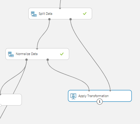
This way, we are telling ML Studio to apply, to the holdout dataset, the same normalize transform used for the training dataset. This is very important because our model has been trained on transformed data and the same transformation must be used in every dataset we want our model to score.
Evaluate the performance
In order to calculate the performances of our model in the holdout, we must make the scoring of the dataset. The operation of giving a dataset to a model is called “Scoring”. The model takes the dataset and returns its prediction, which is a probability that the event labeled with 1 occurs. This probability (called “score”), compared with the real occurring events in the holdout dataset (which the model doesn’t know) will make us evaluate model performance.
In order to score the dataset, we can search for the “Score model” node.

Then, we can add it to the workflow in this way.

The first input port is the trained model (i.e. the output of the Train model node), while the second input port is the dataset to score (in our case, the transformed holdout dataset).
After executing the score model node, we can take a look at what it does.

As you can see, there is a new pair of columns called “Scored Labels” and “Scored Probabilities”. The second one is the probability that the target label is 1, while the first one is the predicted target itself, calculates as 1 if the probability is greater than 50% and 0 otherwise.

Finally, we can use the “Evaluate Model” node to extract the performance metrics we need.

We can connect the score model node to the evaluation node and run it.

Finally, these are the results.

The panel on the left is the ROC curve, which is pretty amazing.
Scrolling down, we can find all the numbers we are looking for.

On the upper left part, we have the confusion matrix. Next, we have the standard metrics for a binary classification model (Accuracy, Precision and so on). The right slider changes the threshold that transforms the probability in the 0–1 label. When you change the threshold, all the metrics change automatically, except for the AUC, which is threshold-independent.
We can say that our model is wonderful (high AUC, high precision, high accuracy), so we can save it inside ML Studio to use it in other experiments.

Conclusion
In this short article, I’ve shown a simple example of the use of Azure ML studio. It’s a very useful tool in the machine learning industry and, although it has some limits (limited number of records, limited choice of models), I think that even the most code-oriented data scientist will love this simple tool. It’s pretty worth mentioning that, paying the appropriate fee, ML studio can be used for real-time training and prediction thanks to its strong REST API interface. This enables many possible machine learning scenarios.