What they are. When they are useful. How they relate to each other.
Consider the data set
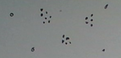
What do you see? I see three definite clusters and 4 outliers. What makes the clusters ‘definite’? Each is dense with many points in it. What makes the singleton clusters outliers? Each is a singleton and far from any of the dense clusters.
Density-based clustering is an approach that fits this example. Its aim is to find maximal clusters, each sufficiently dense. Maximal just means a cluster cannot be grown without decreasing the density significantly. For example, growing the rightmost dense cluster in the figure above by adding the point near the top right corner would decrease the density significantly, so we leave it out, preferring to think of it as an outlier instead.
Once the clusters have been found, clusters that have very few points in them can be deemed outliers.
Before diving into density-based clustering, let’s ask the question: why not use K-means clustering? We’ll assume the reader is familiar with this algorithm. If not, check out [1].
K-means clustering is ill-suited to this problem. For one, what K would you use? Think of it this way. Imagine that as we sampled from the data’s population, the three dense clusters remained largely the same but the outliers changed, including the number of them. This is a reasonable model of a population that inherently forms a small fixed number of clusters but is prone to large random errors, i.e. has an unknown number of outliers.
Using K-means clustering in the above setting would be very sensitive to the choice of K. This is because the total number of clusters can vary significantly from sample to sample. However, the number and characteristics of the dense clusters largely remain the same. So in principle, a density-based approach would be more robust.
Okay, at an intuitive level, the notion of dense clusters is simple and clear. But how do we actually find the dense clusters?
Let’s view the situation as follows. For a given distance d we can define a graph whose edges capture pairs of points that are at most distance d apart. That is, the points are the nodes of this graph. Two points are connected by an edge if they are within distance d.
How does this help us? If we can somehow just choose the right d, the graph’s connectivity structure will capture the cluster structure. This is depicted in the example below.
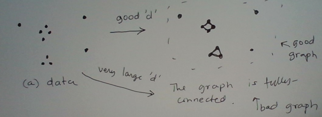
For just the right choice of d, we get a good graph. That is a graph that captures the clusters. When d is too large, the graph is fully-connected (i.e., a clique). This graph is useless for clustering. When d is too small, there may be no edges in the graph. Again, useless for clustering.
Okay so how do we choose a good d? Not an easy question to answer. Still, we’ve made progress. We have transformed the problem into one involving graph clustering. So now we just have to choose a good d. Well, sometimes we can, using domain knowledge or exploratory analysis on the data set. What if neither helps? We’ll defer the discussion on this, to later.
In this particular example, for a good choice of d, the clusters are just the connected components of the graph. (A connected component is a maximal connected piece of the graph.) There are easy algorithms to find the connected components in a graph.
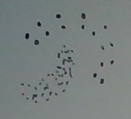
Below is another example on which the connected components algorithm works quite well. This data set has two clusters. Their shapes are such that 2-means clustering wouldn’t work well. (2-means clustering would work better with elliptical clusters.) For the right d, connected components will find these two clusters.
Recap
Okay, so this is what we have so far. If somehow we could choose a good distance threshold d, we can transform the clustering problem into one on graph clustering. Even the simplest graph clustering algorithm, connected components clustering, often works well for the right choice of d.
Viewed this way,
density-based clustering = find good d + graph-based clustering
Beyond Connected Components Clustering
With the right choice of d, connected components clustering can often work quite well. But not always.
Consider the following image.
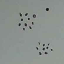
I see two dense clusters plus a singleton cluster (the top right point). (The singleton cluster may be interpreted as an outlier.) With just the right d, the graph’s connected components will mirror these three clusters. However, the range of “right” d’s is quite narrow. With a d even slightly larger, the outlier would be absorbed into its neighboring dense cluster.
Now comes the key point. Even for this d, there is information in the graph that allows us to keep the outlier out of the dense cluster. Specifically, the outlier has degree 0. (The degree of a node is the number of edges in the graph that touch it.) By contrast, each of the nodes in the dense cluster has a degree of at least three.
Okay, so why don’t we replace the “connected component” property with a more stringent “dense subgraph” property. There are different ways we could define “dense subgraph”. One is to require that the number of edges in the subgraph is a certain minimum percentage of the number of edge slots in the subgraph. (An edge slot is a slot in which an edge can fit.) A different way to define “dense subgraph” is to require that every node in the subgraph has a certain minimum degree within the subgraph. The latter is a stricter definition as it requires each of the nodes to have a minimum density. The former only requires the entire subgraph to have a certain minimum density.
In principle, we can partition the graph into maximal subgraphs each of which is sufficiently dense according to whatever definition of “dense” we have chosen. In practice, these types of partitioning problems are generally intractable. That is, very time consuming to solve for large graphs.
This is where heuristic algorithms come in.
DBScan
This is a widely-used density-based clustering method. it heuristically partitions the graph into subgraphs that are dense in a particular way.
It works as follows. It inputs the graph derived using a suitable distance threshold d chosen somehow. The algorithm takes a second parameter D. Any node in the graph whose degree is at least D is termed a core node. A core node is called such because it will form the core of a cluster.
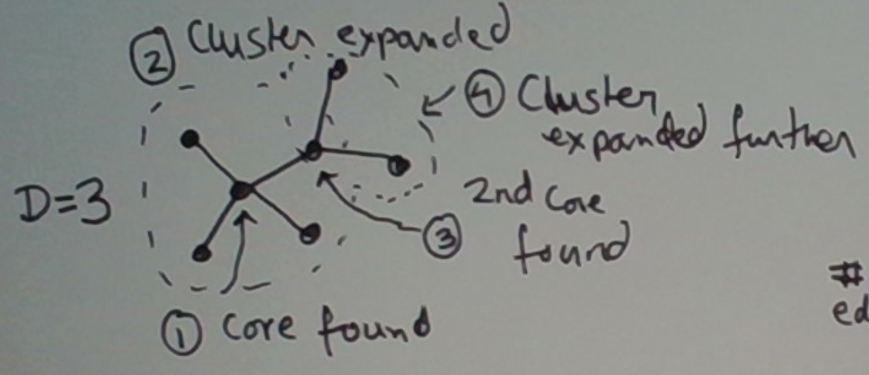
For a given choice of D, the approach works as follows. First, we find the highest-degree node u in the graph. We start a new cluster at this node. Next, we expand this cluster to contain the neighbors of u. Next, if any neighbor v of u is a core node (this is where D comes in) we add the neighbors of v to this same cluster. We keep going until the cluster stops growing. We then freeze the cluster, and repeat this process on the remainder of the graph.
This process is depicted below. In step 1, we find the first core which becomes a new cluster. This core’s degree is 4, which is greater than our setting D = 3. In step 2, we expand this core to include its neighbors into the cluster. This is shown by the dashed circle. In step 3, we discover that one of these neighbors is itself a core. In step 4, we expand out the cluster further to include the neighbors of the second core. So the entire graph shown is now in a single cluster.
Once we have found all the clusters, we deem the ones with sufficiently-many points in them to be dense and the rest to be outliers.
An Alternative Visualization
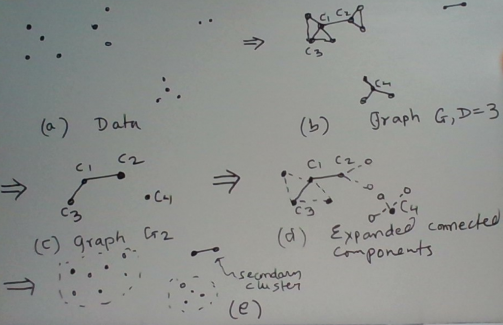
One way to visualize this process is to imagine that from the first graph (which was derived from the data for a given d) we derive a second graph. The nodes of the second graph are the core nodes in the first graph. Two nodes in the second graph are connected by an edge if there is an edge between the same two nodes in the first graph.
Now we find the connected components in the second graph. Each of the resulting clusters contains one or more (core) nodes. We then expand out each of these clusters further using the edges in the original graph. Specifically for every core node in a cluster, we also put its neighbors in the same cluster.
This process may be summarized as follows.
- Build G2 from G.
- Find connected components in G2.
- Expand each connected component using the edges in G.
- If some nodes in G are still unassigned, find connected components in the subgraph of G induced by these nodes. These connected components become additional clusters. Moreover, we also know that these clusters are ‘secondary’ clusters as they don’t have any core points in them.
This view opens the door to using connected component algorithms or implementations.
We illustrate this process in the figure below.
Choosing the Hyperparameters
So the graph-based clustering has one hyperparameter d. DBscan’s particular algorithm has a second: D. How might we choose these when we have no domain knowledge to guide us?
There is no magical algorithm to find the best values. That said, there are some heuristic ways that ease the burden of finding good candidates. We will focus on d, which is more important as it defines the graph.
The number of edges in the graph is a monotone function of d. When d is smaller than the minimum distance between two points in the data set, there is no edge. As we increase d, we start creating edges. Eventually, when d is large enough, we get a fully-connected graph.
Consider this approach. Track the number of edges as a function of d, and pick the first d where there is a significant jump. This is depicted below.
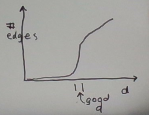
The intuition behind this is that if there are dense clusters in the data, the graph will suddenly get a lot of edges as d approaches the right value.
Consider the example below. It’s not hard to visualize the d at which suddenly lots of edges emerge.

In fact, the graph of the number of edges as a function of d for this picture might look like this.
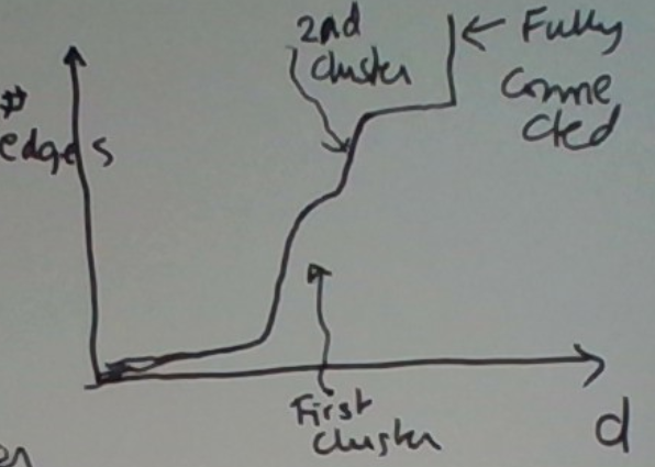
This is because the first cluster is a bit denser than the second one.
HCS
This may be viewed as a conservative variant of connected components clustering (CCC). To see this let’s rename CCC to connected subgraphs clustering. (This is just semantics.) HCS stands for highly connected subgraphs clustering.
Naming aside, how does HCS work? (Previously we said this type of clustering is generally intractable.) It uses the notion of min-cuts. There are many heuristic algorithms to find min-cuts or approximations.
HCS starts with the entire graph and checks if it is highly connected. We can define highly connected however we like so long as we can test for this condition efficiently. If the graph is not highly connected, it partitions the graph into two non-empty subgraphs in such a way that the number of edges that cross the partition is minimized. We might possibly add more constraints on the two graphs. Such as neither is relatively too small, i.e. the partition is not too imbalanced. Such a set of edges is called a min-cut. There are algorithms to find min-cuts under additional constraints. We won’t discuss these.
We then recurse on the two subgraphs.
CCC may be viewed as a special case in which the highly connected condition is just connected and the min-cut must be of size 0.
Example
Consider the graph depicted below. For an appropriate definition of “highly connected”, HCS should find the two clusters below. There is only one edge crossing the clusters. That is, the cut is small.
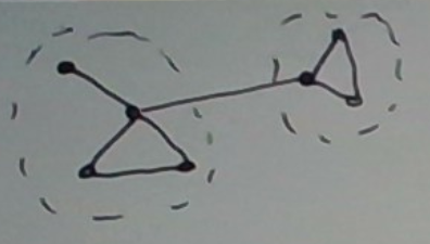
One could reasonably make the case that the top node in the first cluster — the one whose degree is 1 — should go into its own (singleton) cluster. For an appropriate definition of “highly connected,” this can be made to happen.
Summary
In this post, we covered density-based clustering and explained that it is a better fit than K-means clustering to scenarios in which (i) the number of clusters is not known in advance, (ii) there are outliers, and (iii) the clusters are not elliptical.
During the process, we also revealed that more generally graph-based clustering has these attractive properties. In fact, the most popular algorithm for density-based clustering, DBSCAN, is graph-based.
Finally, we covered DBSCAN and a few other graph-based clustering algorithms (CCC, HCS) in some detail.