Basics Of Deep Learning
TL;DR: Have you even wondered what is so special about convolution? In this post, I derive the convolution from first principles and show that it naturally emerges from translational symmetry.
La connoissance de certains principes supplée facilement à la connoissance de certains faits. (Claude Adrien Helvétius)
During my undergraduate studies, which I did in Electrical Engineering at the Technion in Israel, I was always appalled that such an important concept as convolution [1] just landed out of nowhere. This seemingly arbitrary definition disturbed the otherwise beautiful picture of the signal processing world like a grain of sand in one’s eye. How nice would it be to have the convolution emerge from first principles rather than have it postulated! As I will show in this post, such first principles are the notion of translational invariance or symmetry.
Let me start with the formula taught in basic signal processing courses defining the discrete convolution [2] of two n-dimensional vectors x and w:

Here, for convenience, I assume that all the indices run from zero to n−1 and are modulo n; it is convenient to think of vectors as defined on a circle. Writing the above formula as a matrix-vector multiplication leads to a very special matrix that is called circulant:
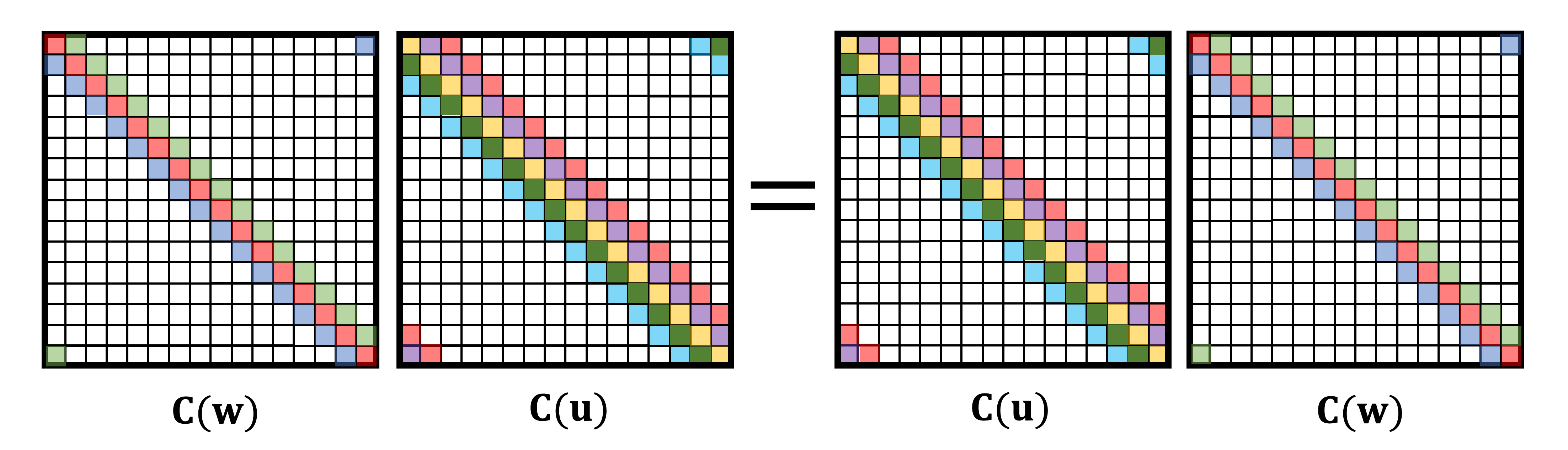
One of the first things we are taught in linear algebra is that matrix multiplication is non-commutative, i.e., in general, AB≠BA. However, circulant matrices are very special exception:
Circulant matrices commute,
or in other words, C(w)C(u)=C(u)C(w). This is true for any circulant matrix, or any choice of u and w. Equivalently, we can say that the convolution is a commutative operation, x∗w=w∗x.
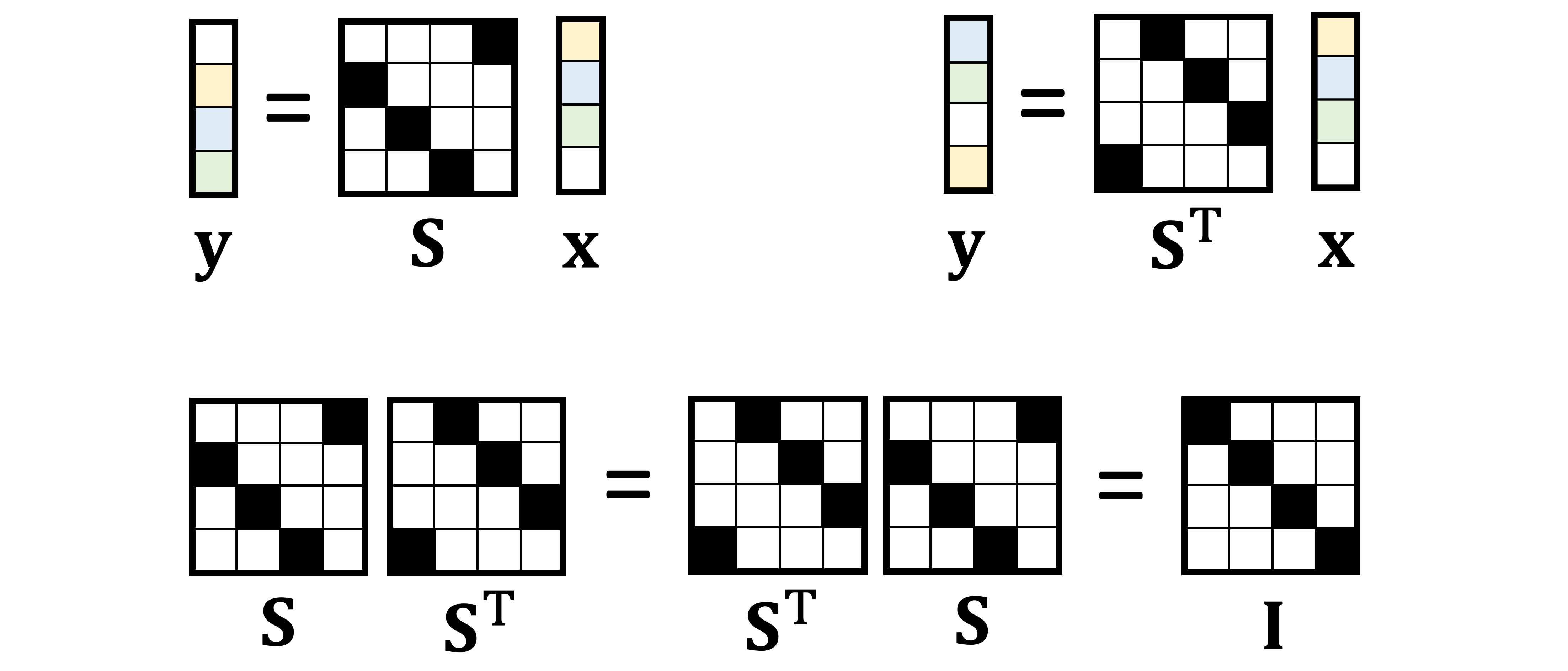
A particular choice of w=[0,1,0…,0] yields a special circulant matrix that shifts vectors to the right by one position. This matrix is called the (right) shift operator [4] and denoted by S. The transpose of the right shift operator is the left shift operator. Obviously, shifting left and then right (or vice versa) does not do anything, which means S is an orthogonal matrix:
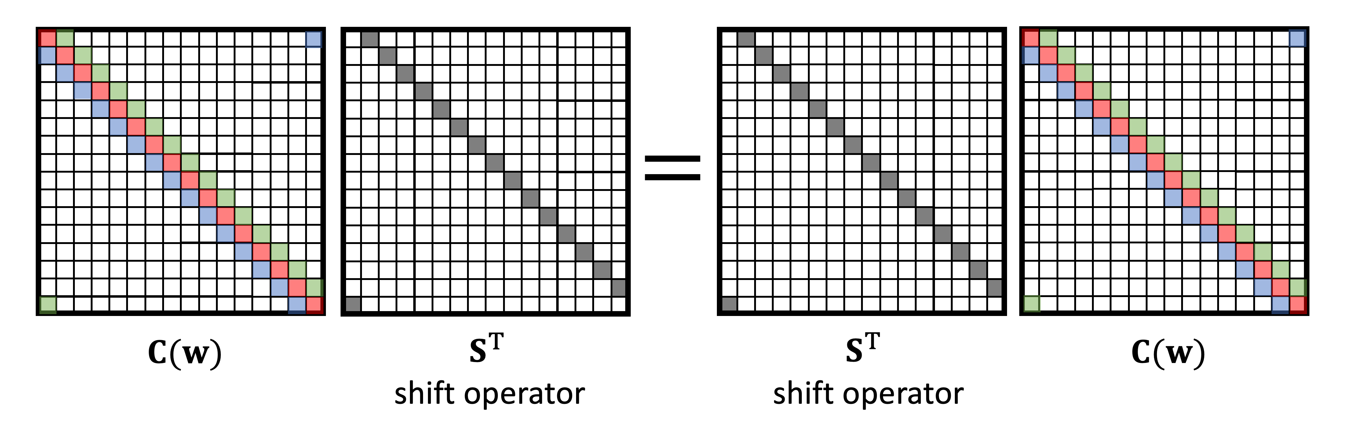
Circulant matrices can be characterised by their commutativity property. It appears to be sufficient to show only commutativity with shift (Lemma 3.1 in [5]):
A matrix is circulant if and only if it commutes with shift.
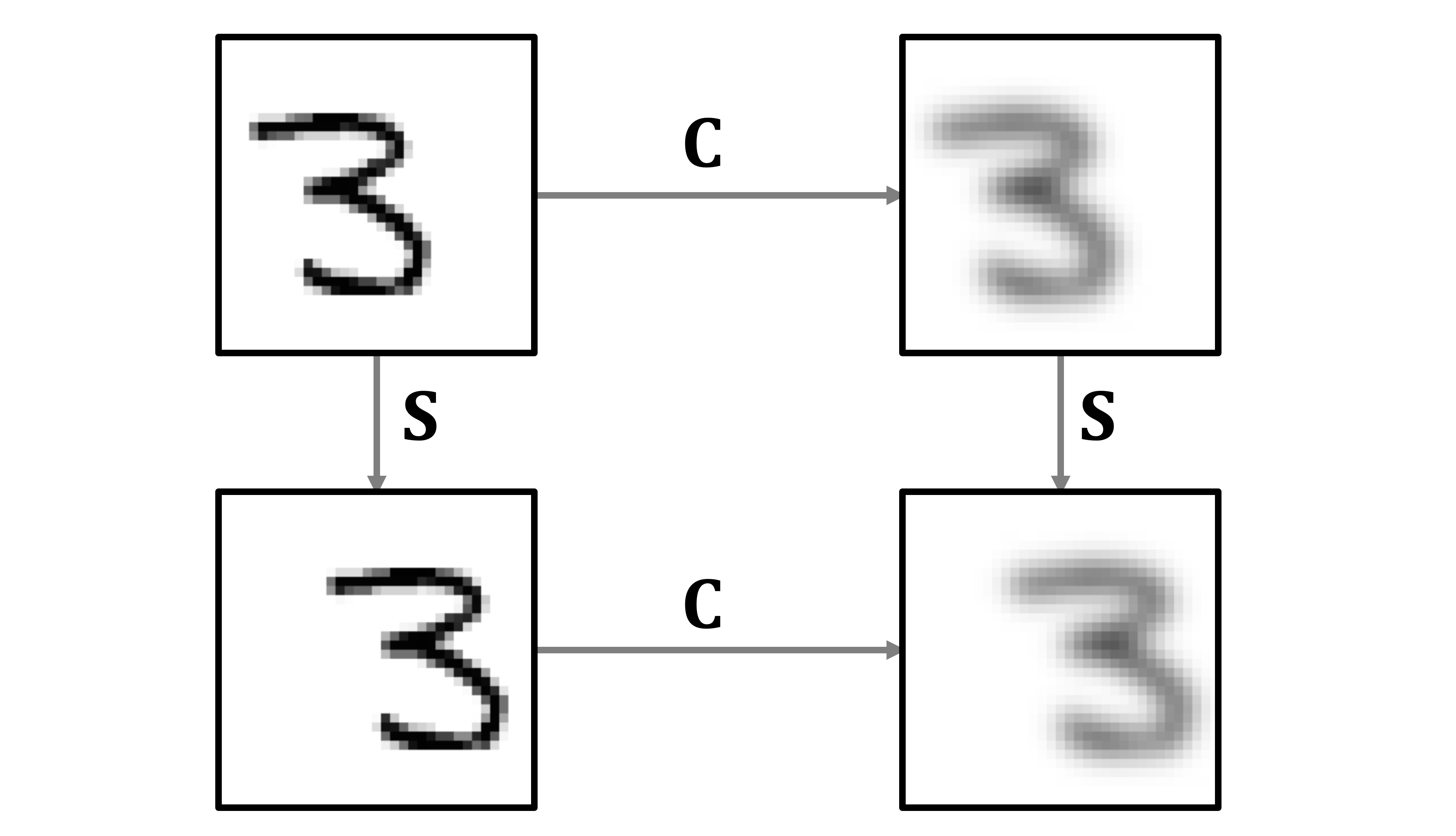
The first direction of this “if and only if” statement leads to a very important property called translation or shift equivariance [6]: the convolution’s commutativity with shift implies that it does not matter whether we first shift a vector and then convolve it, or first convolve and then shift — the result will be the same.
The second direction allows us to define convolution as the shift-equivariant linear operation: in order to commute with shift, a matrix must have the circulant structure. This is exactly what we aspired to from the beginning, to have the convolution emerge from the first principles of translational symmetry [7]. Instead of being given a formula of the convolution and proving its shift equivariance property, as it is typically done in signal processing books, we can start from the requirement of shift equivariance and arrive at the formula of the convolution as the only possible linear operation satisfying it.
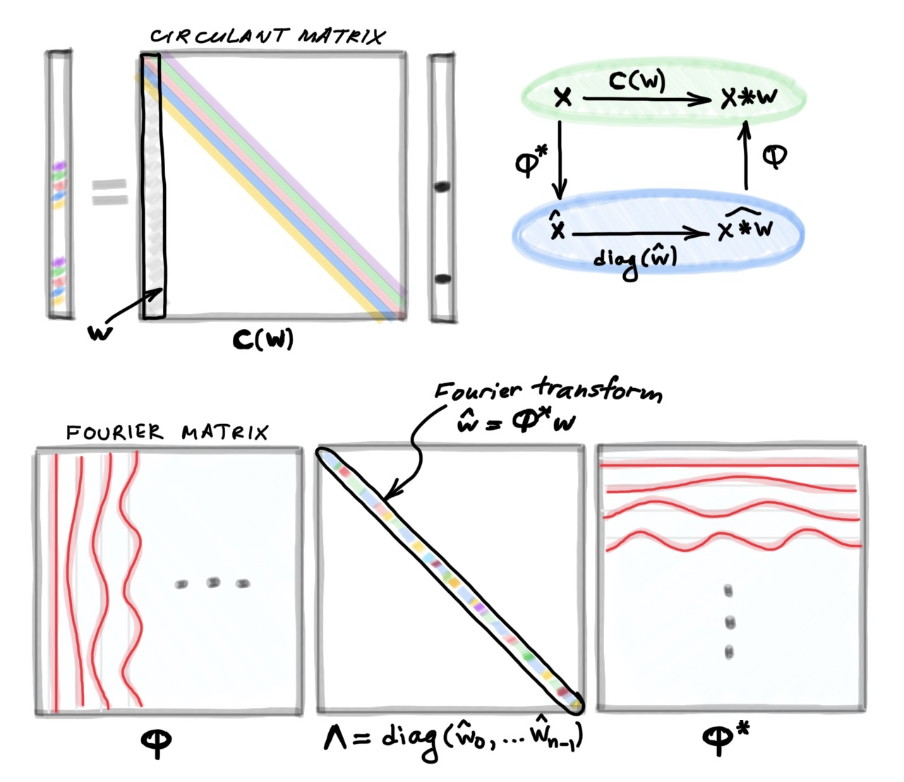
Another important fact taught in signal processing courses is the connection between the convolution and the Fourier transform [8]. Here as well, the Fourier transform lands out of the blue, and then one is shown that it diagonalises the convolution operation, allowing to perform convolution of two vectors in the frequency domain as element-wise product of their Fourier transforms. Nobody ever explains where these sines and cosines come from and what is so special about them.
In order to get to the bottom of it, recall a fact from linear algebra:
Commuting matrices are jointly diagonalisable.
In other words, two matrices satisfying AB=BA will have the same eigenvectors (but possibly different eigenvalues) [9]. Since all circulant matrices commute, we can pick one of them and compute its eigenvectors — the above theorem assures that these will be the eigenvectors of all circulant matrices as well.
It is convenient to pick the shift operator S. Since S is orthogonal matrix, we expect its eigenvectors to be orthogonal [10]. A simple calculation (see Section 4.1 in [5]) leads to the conclusions that
Shift operator is diagonalised by the Fourier transform.
I hope that at this point you have your second “aha” moment for today: this is where the sines and cosines come from! They are the eigenvectors of the shift operator; I denote them as columns of the matrix Φ. Note that the eigenvectors are complex, so we need to take complex conjugation when transposing Φ. Multiplication (from the left) by Φ* is called the Fourier transform, and by Φ the inverse Fourier transform.

Since all circulant matrices are jointly diagonalisable, they are also diagonalised by the Fourier transform [11]. They differ only in their eigenvalues. The last missing bit is the realisation that
The eigenvalues of C(w) are the Fourier transform of w.
We can now put all the pieces of the puzzle into a statement known as the Convolution Theorem: the convolution x∗w can be computed either as a circulant matrix C(w) applied to x in the original system of coordinate (sometimes this is called “spatial domain” convolution), or in the Fourier basis (“spectral domain”) by first computing the Fourier transform of Φ*x, multiplying it by the Fourier transform of w [12], and then computing the inverse Fourier transform.
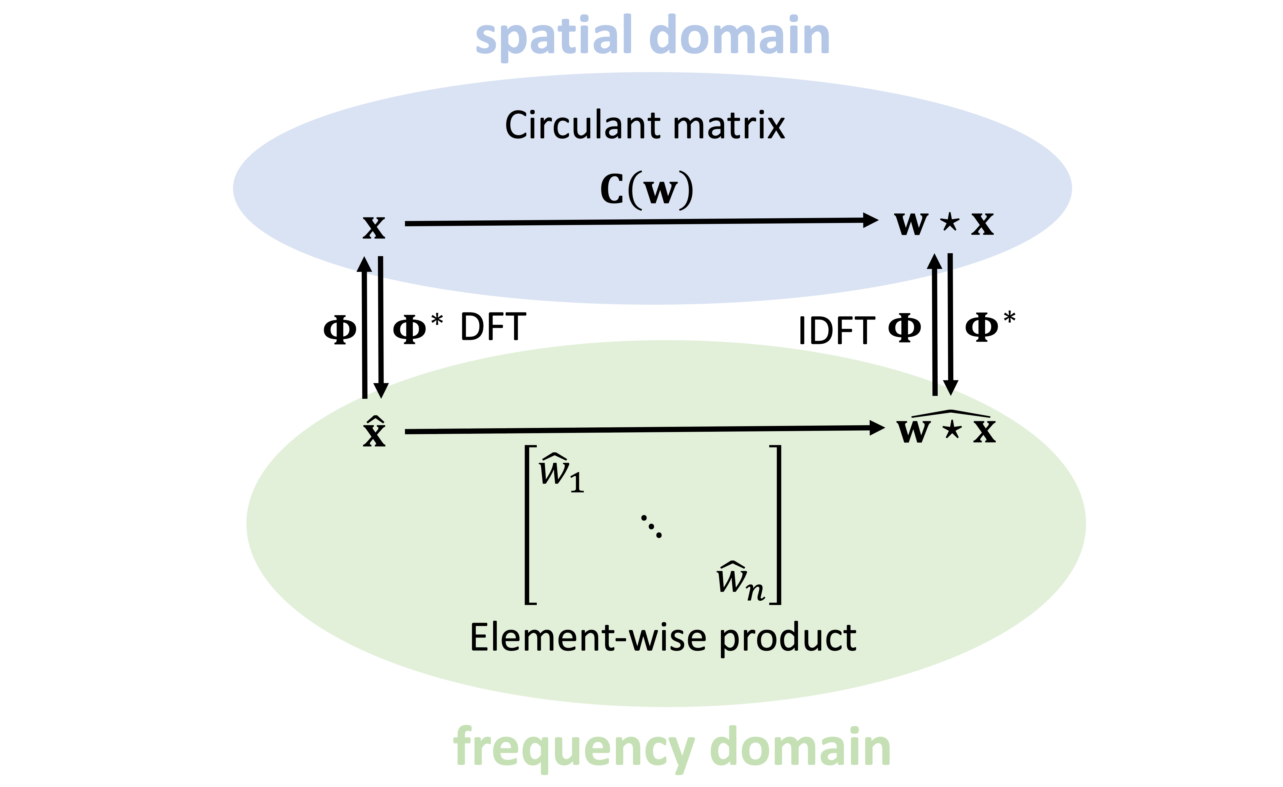
Because Φ has a special redundant structure, the products Φ*x and Φx can be computed with 𝒪(n log n) complexity using a Fast Fourier Transform (FFT) algorithm.
Why is such a definition of convolution a big deal and should be taught this way? I will repeat here the quote from Helvétius I opened this post with: “The knowledge of certain principles easily compensates the lack of knowledge of certain facts”. In the case of convolution, its derivation from first principles allow easy generalisation to other domains. In a next post, I will show how to define convolution on graphs, in order to produce a key building block of graph deep learning architectures.
[1] A. Dominquez-Torres, The history and origins of convolution provides a fascinating excursion into the historical development of the concept and notation of the convolution operation. The convolution integral shows up for the first time in a derivation of Taylor’s theorem in J. B. D’Alembert, Recherches sur différents points importants du système du monde (1754). The priority is often mistakenly attributed to P.-S. de Laplace, Mémoire sur l’inclinaison moyenne des orbites des comètes, sur la figure de la terre et sur les fonctions (1773). Mémoires de l’Académie Royale des Sciences de Paris, Savants Étrangers 7:503–540, though this publication contains no trace of convolution. Laplace indeed used the convolution in his later memoir on probability, written in 1778 and published in 1781. Early naming attempts included résultante (French for “resultant”, first used by Charles Cailler in 1899), composizione (Italian for “composition”, by Vito Volterra in 1910), and faltung (literally meaning “folding” in German, by Gustav Doetsch in 1923); the latter term dominated the German literature in the beginning of the 20th century. The English name convolution comes from the Latin con (“together”) and volvere (“roll up”) and is a literal translation of the German faltung, and so is the Russian variant свёртка. The first use of the English term can be traced to the 1934 paper of Aurel Friedrich Wintner; it was later cemented in the literature by authoritative works of Doetsch (1937) and Gardner and Barnes (1942). The star symbol was first used by Volterra in 1910, though in a different form. Percy John Daniel used a dot notation. The first modern notation of convolution as f∗g, a combination of the two, is due to Doetsch (1923).
[2] Technically speaking, what I define here is circular convolution.
[3] Note that the rows of C(w) have the vector w transposed, resulting in the reflection that appears in the convolution formula and distinguished it from a related notion of correlation. Pay attention to the boundary conditions (the elements of C in the top right and bottom left corners).
[4] I use the terms operator and matrix interchangeably.
[5] B. Bamieh, Discovering transforms: a tutorial on circulant matrices, circular convolution, and the discrete Fourier transform (2018). arXiv:1805.05533 provides the details of the derivations I discuss in this post.
[6] Some often confuse invariance (meaning “unchanged” in Latin) and equivariance (“changing in the same way”), with many signal processing books referring to the property I discuss here as “shift invariance”. A function is shift equivariant if f(Sx)=Sf(x). In other words, it does not matter whether we first apply the shift and then f or vice versa. Differently, shift invariance is the property of being unaffected by shift: the function f(Sx)=f(x) is shift invariant. Shift invariance is a fundamental concept in physics (where it often appears under the name of “translational symmetry”), stating that the laws of physics do not depend on the location in space. In variational formulation of classical mechanics, such a fundamental law as the conservation of momentum follows from shift invariance by virtue of Noether’s theorem.
[7] The concept of equivariance is more general and can be extended using the group theory formalism. This framework was used in T. Cohen and M. Welling, Group equivariant convolutional networks (2016). Proc. ICML, to extend the shift equivariance of convolutional layers of CNNs to more general operations such as rotations. Assuming f : X→Y, where X and Y are some different spaces with corresponding groups 𝒢 and 𝒢’ of operations defined on the elements of X and Y respectively, group equivariance is expressed as f(𝔤(x))=𝔤’(f(x)) where 𝔤∈𝒢 and 𝔤’∈𝒢’. Note that 𝔤’ is not necessarily equal to 𝔤 as the structure and even dimension of the output space Y can be different from that of the input X. The standard convolution discussed in this post is a particular case with X=Y being the space of n-dimensional vectors, 𝒢=𝒢’ the translation group, and 𝔤=𝔤’ the shift operator.
[8] Since we deal with finite-dimensional vectors, the term “Fourier transform” refers here to the Discrete Fourier Transform (DFT).
[9] More precisely, joint diagonalisation implies that two commuting matrices have the same eigenspaces, as in the general case the eigenvalues can have non-trivial multiplicity. Since in the case I discuss here all the eigenvalues are simple, we can talk about a common eigenbasis.
[10] However, since S is non-symmetric, it does not have real eigenvalues (symmetric real matrices have real eigenvalues). The eigenvalues of S happen to be the complex roots of unity.
[11] When I say that matrix C is “diagonalised” by the Fourier transform, I mean that the matrix Φ*CΦ is diagonal. Since Fourier transform is an orthogonal matrix (Φ*Φ=I), geometrically it acts as a change of the system of coordinates that amounts to an n-dimensional rotation. In this system of coordinates, the action of C becomes element-wise product.
[12] In signal processing, one typically designs the filter in the frequency domain, so the Fourier transform of w is never explicitly computed.