A simple explanation and implementation of gradient descent
Let’s say we have a fictional dataset of pairs of variables, a mother and her daughter’s heights:
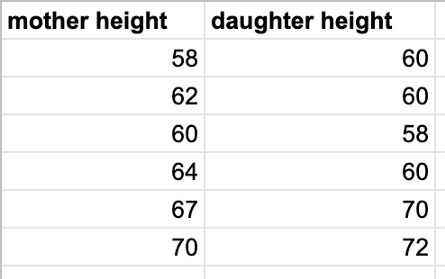
Given a new mother height, 63, how do we predict* her daughter’s height?
The way you do it is by linear regression.
First, you find the line of best fit. Then you use that line for your prediction*.
*Note: I used “predict/prediction” in this article. However, a reader pointed out in the comment below that the correct terminology is “estimate/estimation.”
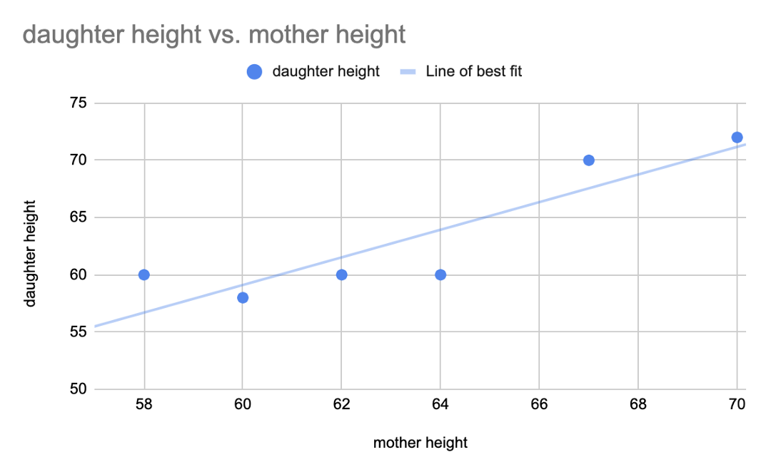
Linear regression is about finding the line of best fit for a dataset. This line can then be used to make predictions.
How do you find the line of best fit?
This is where gradient descent comes in.
Gradient descent is a tool to arrive at the line of best fit
Before we dig into gradient descent, let’s first look at another way of computing the line of best fit.
Statistics way of computing line of best fit:
A line can be represented by the formula: y = mx + b.
The formula for slope m of the regression line is:
m = r * (SD of y / SD of x)
Translation: correlation coefficient between x and y values (r), multiplied by the standard deviation of y values (SD of y) divided by standard deviation of x values (SD of x).
The standard deviation of mothers’ heights in the data above is approximately 4.07. The standard deviation of daughters’ heights is approximately 5.5. The correlation coefficient between these two sets of variable is about 0.89.
So the line of best fit, or regression line is:
y = 0.89*(5.5 / 4.07)x + b
y = 1.2x + b
We know that the regression line crosses the point of averages, so one point on the line is (average of x values, average of y values), or (63.5, 63.33)
63.33 = 1.2*63.5 + b
b = -12.87
Therefore, the regression line as calculated using correlation coefficient and standard deviations is approximately:
y = 1.2x - 12.87
Regression line using statistics is y = 1.2x -12.87
Now, let’s dig into gradient descent.
Gradient descent way of computing line of best fit:
In gradient descent, you start with a random line. Then you change the parameters of the line (i.e. slope and y-intercept) little by little to arrive at the line of best fit.
How do you know when you arrived at the line of best fit?
For every line you try — line A, line B, line C, etc — you calculate the sum of squares of the errors. If line B has a smaller value than line A, then line B is a better fit, etc.
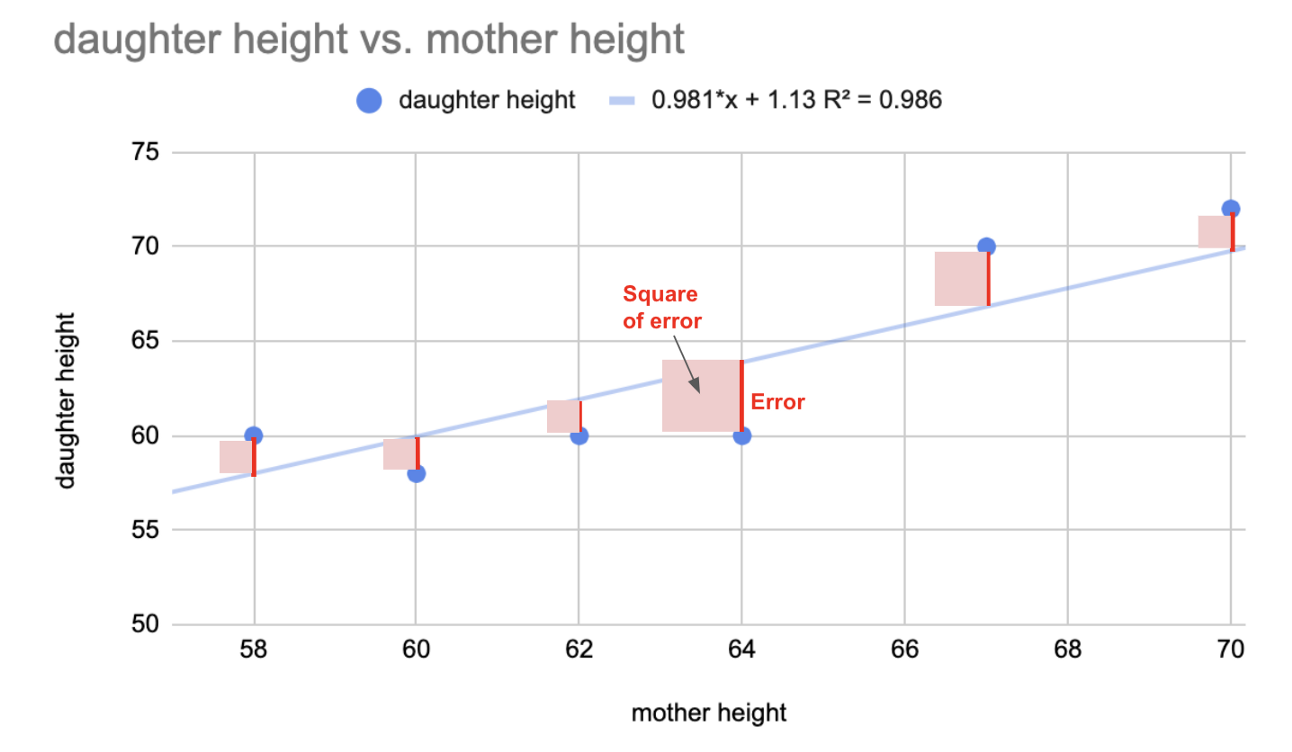
Error is your actual value minus your predicted value. The line of best fit minimizes the sum of the squares of all the errors. In linear regression, the line of best fit we computed above using correlation coefficient also happens to be the least squared error line. That’s why the regression line is called the LEAST SQUARE REGRESSION LINE.
Line of best fit is the least square regression line
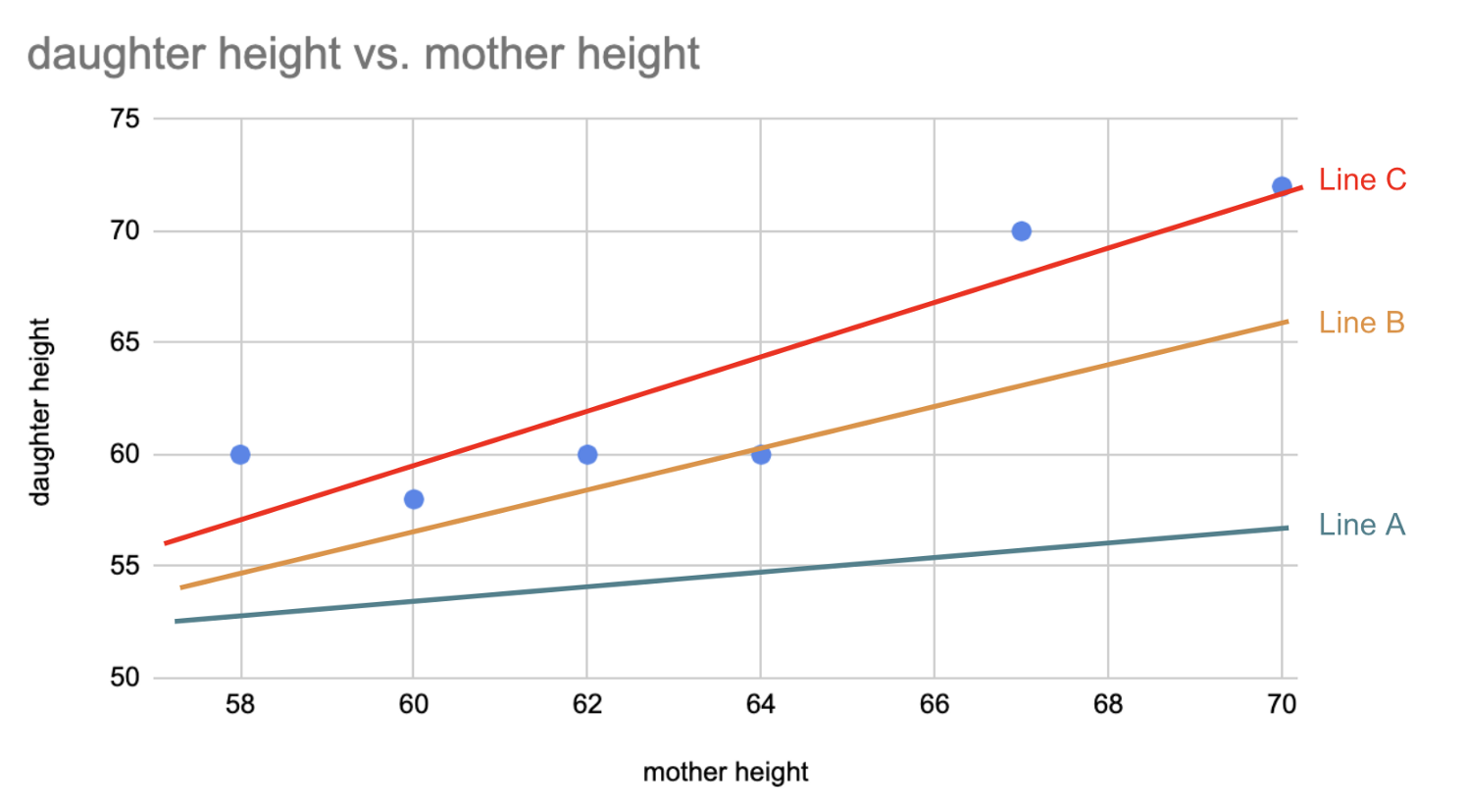
In the image below, line C is better fit than line B, which is better fit than line A.
At a high level, this is how gradient descent works:
You start with a random line, let’s say line A. You compute the sum of squared errors for that line. Then, you adjust your slope and y-intercept. You compute the sum of squared errors again for your new line. You continue adjusting until you reach a local minimum, where the sum of squared errors is the smallest and additional tweaks does not produce better result. The way you adjust your slope and intercept will be covered in more details momentarily.
Gradient descent is an algorithm that approaches the least squared regression line via minimizing sum of squared errors through multiple iterations.
Gradient Descent Algorithm
In machine learning terminology, the sum of squared error is called the “cost”. This cost equation is:
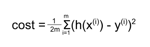
Where:
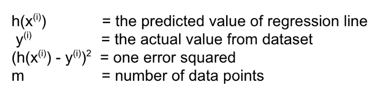
This equation is therefore roughly “sum of squared errors” as it computes the sum of predicted value minus actual value squared.
The 1/2mis to “average” the squared error over the number of data points so that the number of data points doesn’t affect the function. See this explanation for why we divide by 2.
In gradient descent, the goal is to minimize the cost function. We do this by trying different values of slope and intercept. But which values to try and how do you go about changing those values?
We change their values according to the gradient descent formula, which comes from taking the partial derivative of the cost function. The exact math can be found in this link.
By taking the partial derivative, you arrive at the formula:
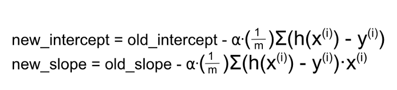
This formula computes by how much you change your theta with each iteration.
The alpha (α) is called the learning rate. The learning rate determines how big the step would be on each iteration. It’s critical to have a good learning rate because if it’s too large your algorithm will not arrive at the minimum, and if it’s too small, your algorithm will take forever to get there. For my example, I picked the alpha to be 0.001
To summarize, the steps are:
- Estimate θ
- Compute cost
- Tweak θ
- Repeat 2 and 3 until you reach convergence.
Here’s my implementation for simple linear regression using gradient descent.
I started at 0,0 for both the slope and intercept.
Note: In machine learning, we use theta to represent the vector [y-intercept, slope]. Theta0 = y-intercept. Theta1=slope. That’s why you see theta as variable name in the implementation below.
Using this algorithm and the dataset above for mothers and daughters heights, I got to a cost of 3.4 after 500 iterations.
The equation after 500 iterations is y = 0.998x + 0.078. The actual regression line is y = 1.2x -12.87 with cost of approximately 3.1.
With an estimate of [0,0] as initial value for [y-intercept, slope], it’s impractical to get to y = 1.2x -12.87 . To get close to that without tons and tons of iterations, you’d have to start with a better estimate.
For example, [-10, 1] will get roughly y = 1.153x — 10 and cost of 3.1 after less than 10 iterations.
Adjusting parameters like learning rate and starting estimate is commonplace in the world of machine learning.
There it is, the gist of gradient descent in linear regression.
Gradient descent is an algorithm that approaches the least squared regression line via minimizing sum of squared errors through multiple iterations.
So far, I’ve talked about simple linear regression, where you only have 1 independent variable (i.e. one set of x values). Theoretically, gradient descent can handle n number of variables.
I’ve refactored my previous algorithm to handle n number of dimensions below.
Everything is the same, the only exception is that instead of using mx + b (i.e. slope times variable x plus y-intercept) directly to get your prediction, you do a matrix multiplication. See def get_prediction in the gist above.
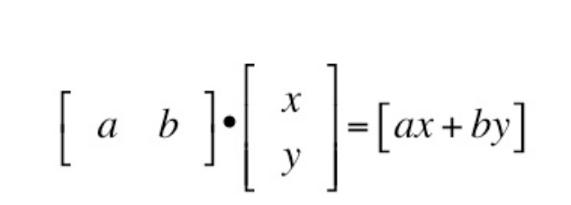
With dot product, your algorithm can take in n number of variables to compute a prediction.
Thank you for reading! Comment below if you have questions!