Fully-connected versus Convolutional
Like other organisms, artificial neural networks have evolved through the ages. In this post, we cover two key anatomies that have emerged: fully-connected versus convolutional. The second one is better suited to problems in image processing in which there are local features in a space with geometry. The first one is generally appropriate on problems in which there isn’t a geometry and spatial locality of features is not paramount.
Single Neurons
Let’s start with models of single artificial neurons, the “Leggo bricks” of neural networks. A neuron takes a vector x as input and derives a scalar output y from it. Most neuron models conform to y = f(wx + b). Here w is the vector of weights of the same dimensionality as x, and b is a scalar called the neuron’s bias. This is graphically depicted below.
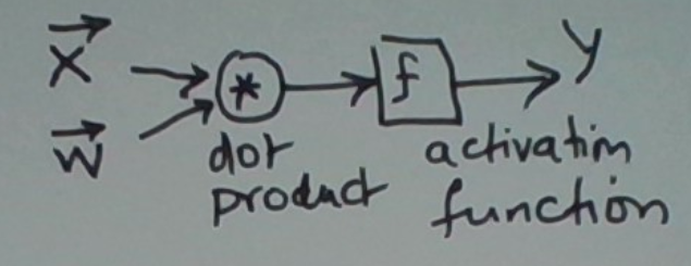
The configurable part of this is the neuron’s activation function f. Different choices of f lead to neurons with quite different capabilities.
The most common choices are linear: f(u) = u, step: f(u) = sign(u), and sigmoid: f(u) = 1/(1+e^-u). These are depicted below.
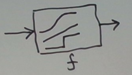
When the target output y is expected to be (approximately) a linear function of x, a linear activation function is called for. This is the setting of linear regression.
When the target output y is binary, we have a choice: a sigmoidal activation function or a step activation function. Both theory and practice favor the sigmoid.
There are several reasons for this.
One is that the sigmoid is differentiable whereas the step function is not. This allows the neuron’s parameters (the weights w and the bias b) to be trained via gradient descent on a data set of input-output pairs.
A second one is that using a sigmoid captures more information which can often be used profitably. For example, consider two situations, one in which the neuron’s output is 0.9 and one in which it is 0.7. We might be inclined to classify both as 1s. (Remember we seek a binary output.) Should we do so, it makes sense to attach higher confidence to the first one since the neuron’s output was higher.
Another way we can use the additional information in the neuron’s output is by adjusting the binary classification threshold. This lets us become more (or less) conservative in our decision-making.
The key point here is that the classification threshold can be adjusted post-training. In fact, any time we wish to. (This is especially useful after the neuron starts making decisions in the “field” and we realize we’d like to tweak its behavior.) This threshold is not a parameter during training. Only the weight vector w and bias b are.
Simply put, if we observe the neuron is overly sensitive (i.e. its outputs are sometimes towards 1 when the target is 0) we can increase the classification threshold. Similarly, if the neuron is not sensitive enough, we can decrease the classification threshold.
Networks of Neurons
Well, actually a single neuron is already an example. A useful one at that. It can be used to map a vector of inputs to a numeric or binary output. That is, to solve regression and binary classification problems.
Often, not very well though.
The first breakthrough is an intermediate layer of neurons between the input and the output. This is graphically depicted below.
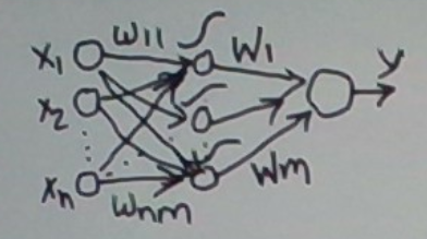
The intermediate layer is called a hidden layer. In the schematic, we have used sigmoidal neurons in the internal layer. Linear hidden neurons are less useful and step neurons have issues we discussed earlier.
A sigmoidal hidden neuron may be viewed as representing some binary feature of the input. The neuron’s value is derived from the input vector x. This value may be viewed as the probability that the associated feature is present in the input.
A neural network with a hidden layer maps an input vector to a vector in a space of features. This mapping is nonlinear. The feature vector is then mapped to the output. This indirect approach results in an architecture that is in principle more powerful than one without the hidden layer.
In practice, there are some issues. How many neurons should go into the hidden layer? This depends on the complexity of the input-to-output mapping problem. This complexity may not be known. For linear problems, we may not need any hidden neurons. In fact, having them might hurt.
The short answer is we don’t. That said, we could try a different number of hidden neurons and pick the one that works best or at least adequately.
On to the next question. For a fixed number of hidden neurons, how do the features they represent get learned? The short answer is via the learning process, typically a form of gradient descent called back-propagation. We won’t go into the details here.
That said, we will depict the roles the various weights touching a hidden neuron play.
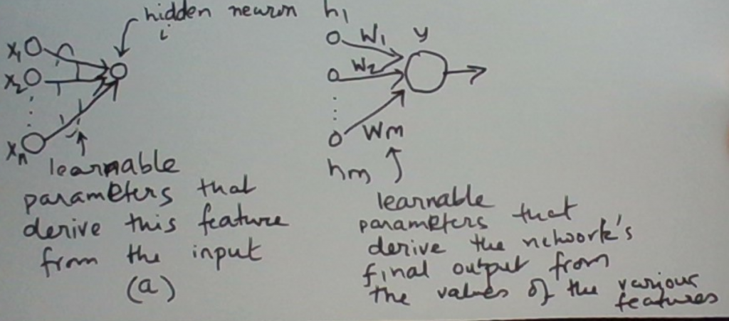
Finally, let’s mention that, as before, the output neuron is sigmoidal for a binary classification problem and linear for a regression problem.
Image Classification Problems
Say we have a large set of images, some containing cats, others not. We’d like to learn a classifier that can tell whether or not an image has a cat in it.
Say each of our images has lots of pixels in them. 100 X 100 = 10,000 for concreteness.
In principle, we could map this problem to a neural network with one hidden layer, as depicted below.
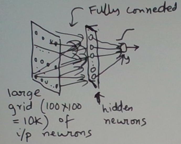
In practice this approach has difficulties. We have 10,000 input neurons. With a hidden layer of m neurons, this means we have 10000*m input-to-hidden weights. It’s hard to imagine that we could use less than 20 hidden neurons to adequately learn a cat-or-not classifier.
20 hidden neurons means 200,000 input-to-hidden weights. That’s a lot of weights to learn! Even with a rich training set, overfitting is a significant risk.
Let’s think differently. Is there structure in this domain (images) that we might be able to exploit? It turns out the answer is yes. First some observations.
- The input neurons are in a spatial grid.
- Features in an image are often local.
- The same feature may occur at different locations in the input.
Let’s expand on 2 and 3. Consider the picture below. It shows horizontal edges at various locations. Each edge is the same feature but at a different location. Each of these feature occurrences is also local. Local just means that to detect the edge at any one location, one only needs to look at pixel values in the proximity of the edge.
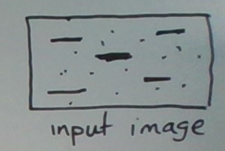
Okay, we now see that each feature is also on the same spatial grid as the input pixels. The implication of this is that for any one feature, there isn’t a single value, rather a grid of values. For each location (i,j), feature f has a value that indicates whether f is present or absent at that location.
Great. Seems like we have gone in the opposite direction. Seems like we have made the problem more complex. Instead of a feature having a single value, it now has a spatial grid of values, one per location.
Not really. How would we try to represent a local feature in an MLNN? Separating out the actual feature function from the location where it applies? Plus, leverage its locality. We can’t.
The inability of the MLNN to (i) exploit feature locality and (ii) the ability to evaluate the feature at many different locations means that we need a lot of hidden neurons to model the combination of the functional and spatial aspects of a feature. (Functional meaning what the feature is, spatial meaning where it is evaluated.) On top of that, because we are unable to exploit locality, the number of input-to-hidden weights explodes.
lots of input neurons X lots of hidden neurons X fully-connected → lots and lots of input-to-hidden weights → Network way overly complex
The picture below depicts the alternative that leverages the input geometry, the locality of features, and the need to evaluate a feature at many different locations.
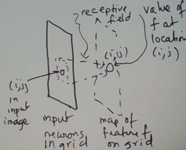
Let’s zoom into the feature’s neuron at location (i,j).
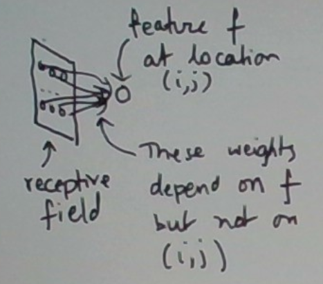
Okay, so any single (local) feature is represented by the same small set of weights. We just slide this feature’s function (called a Kernel) over the various locations (i, j) to get a reading on the feature’s values over the entire grid. This sliding process is called convolution.
By contrast, the MLP has no explicit mechanisms for exploiting either locality or sharing of weights.
Summary
We have covered the anatomical structures of the two most important (feedforward) neural network architectures: fully-connected multi-layer neural networks and convolutional neural networks. We have discussed why convolutional neural networks are better suited to image processing than multi-layer neural networks. On the MLNNs are well-suited to problems in which locality and convolutions don’t come into play in obvious ways.
Further Reading


