What do we want to optimize for? Most of the businesses fail to answer this simple question.
Every business problem is a little different, and it should be optimized differently.
We all have created classification models. A lot of time we try to increase evaluate our models on accuracy. But do we really want accuracy as a metric of our model performance?
What if we are predicting the number of asteroids that will hit the earth.
Just say zero all the time. And you will be 99% accurate. My model can be reasonably accurate, but not at all valuable. What should we do in such cases?
Designing a Data Science project is much more important than the modeling itself.This post is about various evaluation metrics and how and when to use them.
1. Accuracy, Precision, and Recall:
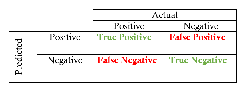
A. Accuracy
Accuracy is the quintessential classification metric. It is pretty easy to understand. And easily suited for binary as well as a multiclass classification problem.
Accuracy = (TP+TN)/(TP+FP+FN+TN)
Accuracy is the proportion of true results among the total number of cases examined.
When to use?
Accuracy is a valid choice of evaluation for classification problems which are well balanced and not skewed or No class imbalance.
Caveats
Let us say that our target class is very sparse. Do we want accuracy as a metric of our model performance? What if we are predicting if an asteroid will hit the earth? Just say No all the time. And you will be 99% accurate. My model can be reasonably accurate, but not at all valuable.
B. Precision
Let’s start with precision, which answers the following question: what proportion of predicted Positives is truly Positive?
Precision = (TP)/(TP+FP)
In the asteroid prediction problem, we never predicted a true positive.
And thus precision=0
When to use?
Precision is a valid choice of evaluation metric when we want to be very sure of our prediction. For example: If we are building a system to predict if we should decrease the credit limit on a particular account, we want to be very sure about our prediction or it may result in customer dissatisfaction.
Caveats
Being very precise means our model will leave a lot of credit defaulters untouched and hence lose money.
C. Recall
Another very useful measure is recall, which answers a different question: what proportion of actual Positives is correctly classified?
Recall = (TP)/(TP+FN)
In the asteroid prediction problem, we never predicted a true positive.
And thus recall is also equal to 0.
When to use?
Recall is a valid choice of evaluation metric when we want to capture as many positives as possible. For example: If we are building a system to predict if a person has cancer or not, we want to capture the disease even if we are not very sure.
Caveats
Recall is 1 if we predict 1 for all examples.
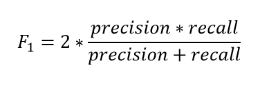
And thus comes the idea of utilizing tradeoff of precision vs. recall — F1 Score.
2. F1 Score:
This is my favorite evaluation metric and I tend to use this a lot in my classification projects.
The F1 score is a number between 0 and 1 and is the harmonic mean of precision and recall.
Let us start with a binary prediction problem. We are predicting if an asteroid will hit the earth or not.
So if we say “No” for the whole training set. Our precision here is 0. What is the recall of our positive class? It is zero. What is the accuracy? It is more than 99%.
And hence the F1 score is also 0. And thus we get to know that the classifier that has an accuracy of 99% is basically worthless for our case. And hence it solves our problem.
When to use?
You can calculate the F1 score for binary prediction problems using:
from sklearn.metrics import f1_score
y_true = [0, 1, 1, 0, 1, 1]
y_pred = [0, 0, 1, 0, 0, 1]

f1_score(y_true, y_pred)# y_pred is an array of predictions
def bestThresshold(y_true,y_pred):
best_thresh = None
best_score = 0
for thresh in np.arange(0.1, 0.501, 0.01):
score = f1_score(y_true, np.array(y_pred)>thresh)
if score > best_score:
best_thresh = thresh
best_score = score
return best_score , best_threshCaveats
The main problem with the F1 score is that it gives equal weight to precision and recall. We might sometimes need to include domain knowledge in our evaluation where we want to have more recall or more precision.
To solve this, we can do this by creating a weighted F1 metric as below where beta manages the tradeoff between precision and recall.
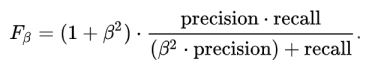
Here we give β times as much importance to recall as precision.
from sklearn.metrics import fbeta_score

y_true = [0, 1, 1, 0, 1, 1]
y_pred = [0, 0, 1, 0, 0, 1]

fbeta_score(y_true, y_pred,beta=0.5)3. Log Loss/Binary Crossentropy
Log loss is a pretty good evaluation metric for binary classifiers and it is sometimes the optimization objective as well in case of Logistic regression and Neural Networks.
Binary Log loss for an example is given by the below formula where p is the probability of predicting 1.
As you can see the log loss decreases as we are fairly certain in our prediction of 1 and the true label is 1.
When to Use?
When the output of a classifier is prediction probabilities. Log Loss takes into account the uncertainty of your prediction based on how much it varies from the actual label. This gives us a more nuanced view of the performance of our model. In general, minimizing Log Loss gives greater accuracy for the classifier.
How to Use?
from sklearn.metrics import log_loss
Caveats
It is susceptible in case of imbalanced datasets. You might have to introduce class weights to penalize minority errors more or you may use this after balancing your dataset.
4. Categorical Crossentropy
The log loss also generalizes to the multiclass problem. The classifier in a multiclass setting must assign a probability to each class for all examples. If there are N samples belonging to M classes, then the Categorical Crossentropy is the summation of -ylogp values:

yijyij is 1 if the sample i belongs to class j else 0
pijpij is the probability our classifier predicts of sample i belonging to class j.
When to Use?
When the output of a classifier is multiclass prediction probabilities. We generally use Categorical Crossentropy in case of Neural Nets. In general, minimizing Categorical cross-entropy gives greater accuracy for the classifier.
How to Use?
from sklearn.metrics import log_loss

# Where y_pred is a matrix of probabilities with shape ***= (n_samples, n_classes)*** and
y_true is an array of class labels
log_loss(y_true, y_pred, eps=1e-15)
Caveats:
The main problem with the F1 score is that it gives equal weight to precision and recall. We might sometimes need to include domain knowledge in our evaluation where we want to have more recall or more precision.
To solve this, we can do this by creating a weighted F1 metric as below where beta manages the tradeoff between precision and recall.
Here we give β times as much importance to recall as precision.
from sklearn.metrics import fbeta_score

y_true = [0, 1, 1, 0, 1, 1]
y_pred = [0, 0, 1, 0, 0, 1]

fbeta_score(y_true, y_pred,beta=0.5)
F1 Score can also be used for Multiclass problems. See this awesome blog post by Boaz Shmueli for details.
3. Log Loss/Binary Crossentropy
Log loss is a pretty good evaluation metric for binary classifiers and it is sometimes the optimization objective as well in case of Logistic regression and Neural Networks.
Binary Log loss for an example is given by the below formula where p is the probability of predicting 1.

As you can see the log loss decreases as we are fairly certain in our prediction of 1 and the true label is 1.
When to Use?
When the output of a classifier is prediction probabilities. Log Loss takes into account the uncertainty of your prediction based on how much it varies from the actual label. This gives us a more nuanced view of the performance of our model. In general, minimizing Log Loss gives greater accuracy for the classifier.
How to Use?
from sklearn.metrics import log_loss

# where y_pred are probabilities and y_true are binary class labels
log_loss(y_true, y_pred, eps=1e-15)
Caveats
It is susceptible in case of imbalanced datasets. You might have to introduce class weights to penalize minority errors more or you may use this after balancing your dataset.
4. Categorical Crossentropy
The log loss also generalizes to the multiclass problem. The classifier in a multiclass setting must assign a probability to each class for all examples. If there are N samples belonging to M classes, then the Categorical Crossentropy is the summation of -ylogp values:
yijyij is 1 if the sample i belongs to class j else 0
pijpij is the probability our classifier predicts of sample i belonging to class j.
When to Use?
When the output of a classifier is multiclass prediction probabilities. We generally use Categorical Crossentropy in case of Neural Nets. In general, minimizing Categorical cross-entropy gives greater accuracy for the classifier.
How to Use?
from sklearn.metrics import log_loss

# Where y_pred is a matrix of probabilities with shape ***= (n_samples, n_classes)*** and
y_true is an array of class labels
log_loss(y_true, y_pred, eps=1e-15)
Caveats:
It is susceptible in case of imbalanced datasets.
5. AUC
AUC is the area under the ROC curve.
What is the ROC curve?
We have got the probabilities from our classifier. We can use various threshold values to plot our sensitivity(TPR) and (1-specificity)(FPR) on the cure and we will have a ROC curve.
Where True positive rate or TPR is just the proportion of trues we are capturing using our algorithm.
Sensitivty = TPR(True Positive Rate)= Recall = TP/(TP+FP)
and False positive rate or FPR is just the proportion of false we are capturing using our algorithm.
1- Specificity = FPR(False Positive Rate)= FP/(TN+FP)
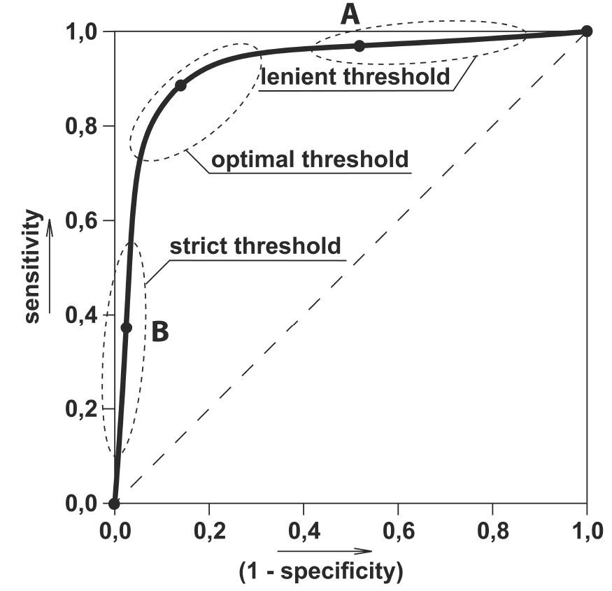
Here we can use the ROC curves to decide on a Threshold value. The choice of threshold value will also depend on how the classifier is intended to be used.
If it is a cancer classification application you don’t want your threshold to be as big as 0.5. Even if a patient has a 0.3 probability of having cancer you would classify him to be 1.
Otherwise, in an application for reducing the limits on the credit card, you don’t want your threshold to be as less as 0.5. You are here a little worried about the negative effect of decreasing limits on customer satisfaction.
When to Use?
AUC is scale-invariant. It measures how well predictions are ranked, rather than their absolute values. So, for example, if you as a marketer want to find a list of users who will respond to a marketing campaign. AUC is a good metric to use since the predictions ranked by probability is the order in which you will create a list of users to send the marketing campaign.
Another benefit of using AUC is that it is classification-threshold-invariant like log loss. It measures the quality of the model’s predictions irrespective of what classification threshold is chosen, unlike F1 score or accuracy which depend on the choice of threshold.
How to Use?
import numpy as np
from sklearn.metrics import roc_auc_score
y_true = np.array([0, 0, 1, 1])
y_scores = np.array([0.1, 0.4, 0.35, 0.8])

print(roc_auc_score(y_true, y_scores))
Caveats
Sometimes we will need well-calibrated probability outputs from our models and AUC doesn’t help with that.
Conclusion
An important step while creating our machine learning pipeline is evaluating our different models against each other. A bad choice of an evaluation metric could wreak havoc to your whole system.
So, always be watchful of what you are predicting and how the choice of evaluation metric might affect/alter your final predictions.
Also, the choice of an evaluation metric should be well aligned with the business objective and hence it is a bit subjective. And you can come up with your own evaluation metric as well.