A practical overview with examples and Python code.
Probability distributions are mathematical functions describing probabilities of things happening. Many processes taking place in the world around us can be described by a handful of distributions that have been well-researched and analyzed. Getting one’s head around these few goes a long way towards being able to statistically model a range of phenomena. Let’s take a look at six useful probability distributions!

Binomial distribution
Arguably the most intuitive yet powerful probability distribution is the binomial distribution. It can be used to model binary data, that is data that can only take two different values, think: “yes” or “no”. This makes the binomial distribution suitable for modeling decisions or other processes, such as:
- Did the client buy the product, or not?
- Did the medicine help the patient to recover, or not?
- Was the online ad clicked on, or not?
Two key elements of the binomial model are a set of trials (binary experiments) and the probability of success (success is the “yes” outcome: an ad clicked on or a patient cured). For instance, the trials may consist of 10 coin flips — each of them is a binary experiment with two possible outcomes: heads or tails. The probability of success, defined as tossing heads, is 50%, assuming the coin is fair.
The binomial distribution can answer the question: what is the probability of observing different numbers of heads in 10 tosses with a fair coin?
https://gist.github.com/MichalOleszak/c302617f785d68e08d00367982a82951#file-binomial-py
Plotting the binomial PMF. Some plot-formatting code has been omitted.
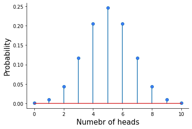
The binomial probability mass function plotted above is the answer! You can see that it’s most likely to observe 5 heads in 10 tosses, and the probability of such an outcome is roughly 25%.
An example of practical usage of the binomial distribution is to model clicks vs non-clicks on an ad banner, where the probability of success is the click-through rate. The binomial distribution may serve as an anomaly detector. Say you have displayed your ad to 750 users and 34 clicked on it. This gives a click-through rate of 4.5%. If you know the average click-through rate for all your previous ads was 6%, you might want to ask: what’s the probability of observing no more than 4.5% this time? To answer this, you can model your clicks with a binomial distribution with the success probability of 6%, which looks like this:
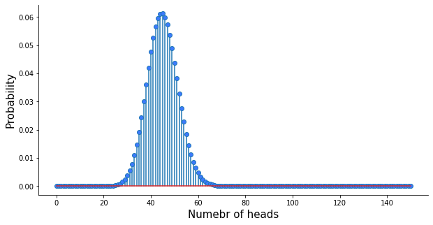
So, what’s the probability of observing no more than 34 clicks in 750 impressions? The answer is the sum of all bars from 0 through 34, or: binom.cdf(34, 750, 0.06) which is 4.88%, quite unlikely. Either the new ad is really bad, or something fishy is happening here… Are you sure your ad provider actually did display it to 750 users?
The binomial distribution describes yes-no data. It may serve as an anomaly detector or a tool for Bayesian A/B testing.
Another common application of the binomial distribution is for Bayesian A/B testing. Imagine you have run two marketing campaigns and want to compare them. A simple comparison of two click-through rates can be misleading, as there is a random component in both, and one can seem higher than the other as a result of chance alone. There are two ways to establish which campaign was better: you can either resort to classical hypothesis testing (more or this later), or explicitly estimate the probability that campaign A was better than campaign B with the Bayesian approach. The latter assumes that the clicks follow the binomial distribution and the calculation of the Bayesian posterior probabilities involves the binomial density formula. How to do this is a topic that deserves a separate treatment, but if you’d like to learn about Bayesian A/B testing or Bayesian statistics in general, I encourage you to take a look at the Bayesian Data Analysis in Python course that I teach on DataCamp.
Poisson distribution
Another very useful distribution is the Poisson distribution. Just like the binomial, it is also a discrete distribution, meaning that it has a limited set of possible outcomes. For the binomial distribution, there were just two: yes or no. For the Poisson distribution, there might be more, but they can only be natural numbers: 0, 1, 2, and so on.
The Poisson distribution can be used to describe events that occur at some rate over time or space. Such processes are everywhere: clients make a purchase in your online store every X minutes, and every Yth product coming off the assembly line is defective.
The Poisson distribution has one parameter, typically denoted with a greek letter λ (lambda), which denotes the rate at which events are happening. The typical use case is to estimate λ from the data and then use the resulting distribution to perform queueing simulations that help allocate resources.
Imagine you have a machine learning model deployed in the cloud and receiving requests from your customers in real-time. How much cloud resources do you need to pay for in order to be 99% sure you can serve all the traffic that arrives at the model in any one-minute period? To answer this question, you first need to know how many requests are coming, on average, in a one-minute period. Say that it’s 3.3 requests on average based on your traffic data. That’s your λ, and hence the Poisson distribution describing your data looks like this:
https://gist.github.com/MichalOleszak/304915120943882da2212065c6cb4125#file-poisson-py
Plotting the Poisson PMF. Some plot-formatting code has been omitted.
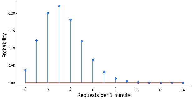
Based on your Poisson distribution, you can calculate the probability of observing 2 events within one minute: poisson.pmf(2, 3.3), which yields 20%, or the probability of getting 5 requests or less: poisson.cdf(5, 3.3) which is 88%.
Poisson distribution describes events that occur at some rate over time od space. It can be used to conduct queueing simulations that help allocate resources.
Cool, but the question was: how many requests per minute do you need to be able to process so that you can be 99% sure to process all the traffic? One way to answer this is to simulate a lot (say, 1,000,000) one-minute periods and calculate the 99th percentile of the number of requests.
https://gist.github.com/MichalOleszak/2fb20c357bfd5e017b57621e1c22b56f#file-simulate_poisson-py
This yields 8, meaning that if you buy enough resources to process 8 requests per minute, you can be 99% sure to process all the traffic in any one-minute period.
Exponential distribution
Another distribution, closely related to Poisson, is the exponential distribution. If the number of events occurring in some time period follows the Poisson process, then the time between those events is described by the exponential distribution.
Continuing the previous example, if we observe 3.3 requests per minute on average, we can model the time between the requests using the exponential distribution. Let’s express it in seconds: 3.3 requests per minute is 0.055 requests per second. One caveat is that in Python’sscipy package, the exponential distribution is parametrized with a scale, which is the inverse of a rate. Also, the exponential distribution is continuous rather than discrete, which means it can take infinitely many values. To emphasize this, we plot it as a shaded area rather than as vertical bars. The distribution in question looks as follows:
https://gist.github.com/MichalOleszak/cb17dd53ff1d19a10b8dcf4a00d7ef81#file-exponential-py
Plotting the exponential PDF. Some plot-formatting code has been omitted.
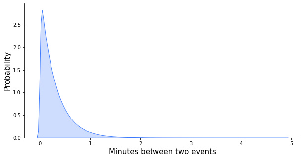
With the average rate of more than three requests per minute, in most cases, there won’t be more than a minute since one request before another one comes in. Sometimes, however, as many as five minutes may pass requestlessly!
Just like the binomial distribution, the exponential distribution can also serve as an anomaly detector. After you haven’t seen a request for 5 minutes, you might start to wonder whether your systems are still alive. What’s the probability of five or more minutes passing without a request? That’s the sum of all bars starting from five and to the right up to infinity, which is equivalent to one minus the bars to the left from five since the sum of all bars must be one. So, it’s 1 — expon.cdf(4, 1/3.3), which is 2.5%. Not very likely, but can happen once in a while.
Exponential distribution can be used as an anomaly detector or as a simple benchmark for predictive models.
Another common use case for the exponential distribution is as a simple benchmark for predictive models. For example, in order to predict when each product will be bought again, you might use gradient boosting or build a fancy neural network. To evaluate their performance, it’s a good practice to compare them against a simple benchmark. If you state your problem as predicting the time until the next purchase, then the exponential distribution is a great benchmark. Once you have the training data (days_till_next_purchase = [1, 4, 2, 2, 3, 6, …, ]), all you have to do is to fit the exponential distribution to these data and take its mean as the prediction:avg, _ = expon.fit(days_till_next_purchase).
Normal distribution
The normal distribution, also known as the bell-curve, is perhaps the most famous one, and also the most widely used — although often implicitly.
First and foremost, the Central Limit Theorem, which is the cornerstone of statistical inference, is all about the normal distribution. I encourage you to read more about it here:Central Limit TheoremOn the relevance of the cornerstone of statistical inference for data scientists.
In a nutshell, the CLT establishes that some statistics, such as a sum or a mean, calculated from random samples of data follow the normal distribution. The two most important practical use cases for the CLT are regression analysis and hypothesis testing.
First, let’s talk regression. In a regression model, the dependent variable is being explained by some predictor variables plus an error term, which we assume to be normally distributed. This assumed normality of error stems from the CLT: we can view the error as the sum of many independent errors caused by omitting important predictors or by random chance. Each of these many errors can have any distribution, but their sum will be approximately normal by the CLT.
Assumption of errors normality in regression models can be justified by the Central Limit Theorem. It is also useful for some hypothesis tests.
Second, hypothesis testing. More elaborate examples will follow shortly when we talk about the chi-square and F distributions. For now, consider this short example: a company specializing in ads retargeting boasts that their precisely targeted ads receive a click-through rate of 20% on average. You run a pilot of 1000 impressions with them and observe 160 clicks, which means the click-through rate of only 16%. Is the targeting not as good, or was it just bad luck?
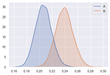
If you consider the 1000 users to whom to ads were displayed a random subset from the larger population of users, then the CLT kicks in and the click-through rate should follow a normal distribution. Assuming the targeting company tells the truth, it should be a normal with a mean of 0.2 and a standard deviation of 0.013. Check out my post on the CLT for the calculations, or just trust me this. The distribution in question looks as follows:
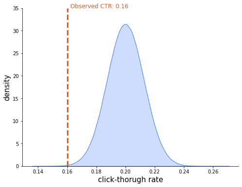
Under this distribution, the 16% click-through rate you have observed is rather improbable, indicating that the alleged 20% average is most likely not true.
Chi-square distribution
The χ2 or chi-square distribution comes in handy in A/B/C testing. Imagine you have conducted an experiment in which you have randomly displayed your website in different color versions to the users. You’re curious which color leads to the most purchases made through the website. Each color has been displayed to 1000 users, and here are the results:
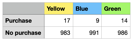
The yellow version seems to be almost twice as good as the blue one, but the numbers are low, so how can you be sure these results are not due to chance?
Hypothesis testing to the rescue! To learn more about the topic, don’t hesitate to take a detour to my Hypothesis Tester’s Guide:The Hypothesis Tester’s GuideA short primer on why can reject hypotheses, but cannot accept them, with examples and visuals.
Here, let me just highlight the role of the chi-square distribution in the process. The first step is to assume that the three website version generate the same number of purchases, on average. If that were to be true, we would expect the same number of purchases for each version, and it would be (17+9+14)/3, or 13.33 purchases. The chi-square distribution allows us to measure how much the observed purchases depart from what’s expected if the color made no difference.
Chi-square distribution is useful for A/B/C testing. It measures how likely it is that the experimental results we got are a result of chance alone.
It turns out that if we compute the (appropriately scaled and then squared) difference between the expected and observed values for each color, we arrive at a test statistic that follows the chi-squared distribution! We can then infer, based on the p-value, whether the variation in the number of purchases we’ve observed was due to chance, or rather indeed due to the color difference.
https://gist.github.com/MichalOleszak/559fdd552cf3266dfb23696c8bdba4ae#file-chi2test-py
This so-called chi-square test is a one-liner in Python:
https://gist.github.com/MichalOleszak/559fdd552cf3266dfb23696c8bdba4ae#file-chi2test-py
Chi-square test for the website color experiment.
We get a chi-square (chisq)value of 2.48 and the distribution is parametrized with 2 degrees of freedom (df). Hence, the distribution in question looks like this:
https://gist.github.com/MichalOleszak/17004d64a2f51bee56eb1d08dcc914b5#file-chi2-py
Plotting the chi-square PDF with 2 degrees of freedom. Some plot-formatting code has been omitted.
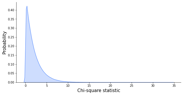
The chi-square value of 2.48 seems pretty likely under this distribution, which leads us to conclude that the differences in the number of purchases for differently-colored websites can be caused by random chance alone. This is further proved by the high p-value of almost 0.3. Please check out the HTG for more on hypothesis testing.
F-distribution
Let’s stick to the website color experiment, an example of A/B/C testing. We have assessed the impact of color on a discrete variable: the number of purchases. Let’s consider a continuous variable now, such as the number of seconds spent, on average, on each website variant.
As part of the experiment, we have randomly shown the users different website variants and we calculated the time they spent on the website. Below are the data for 15 users (five were shown the yellow version, another five the blue one, and the last five the green one). For such an experiment to be valid, we would need many more than 15 users, this is just a demonstration.
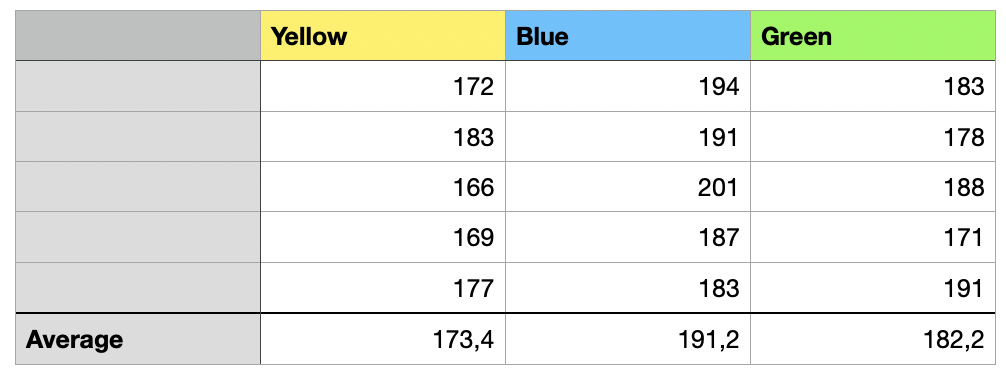
We are interested in the extent to which the differences between the means are larger than what might have been produced by random chance. If they are significantly larger, then we might conclude that the color indeed impacts the time spent on the website. Such a comparison between means is referred to as ANOVA, or analysis of variance.
The inference is quite similar to the one we’ve already discussed when talking about the chi-square distribution. We calculate the test statistic as the ratio between the variability among the group means and the variation within the groups. Such a statistic follows a distribution called the F-distribution. Knowing this, we can use the p-value to reject (or not) the assumption that the means are different due to chance alone.
F-distribution is used for A/B/C testing when the outcome we measure is continuous.
In Python, we can run ANOVA using the statsmodels package. The internal computations are based on a linear regression model, hence the call to ols() and gathering the data into a two-column data frame.
https://gist.github.com/MichalOleszak/63e054a1a66260bc99777034fce3f41b#file-anova-py
Analysis of variance (ANOVA) for the impact of website color on the time spent on it.
And here is the anova_table that we got:
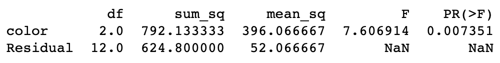
Our F-distribution is parameterized with two degrees-of-freedom parameters: one for differences between the color-means and the grand average (2) and another for the differences within each color (12). Hence, our distribution looks as follows:
https://gist.github.com/MichalOleszak/f17fd2791ac22d313cee6db78e343a98#file-f-py
Plotting the F PDF with 2 and 12 degrees of freedom. Some plot-formatting code has been omitted.
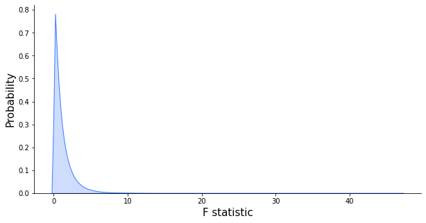
Since we got the F-statistic equal to 7.6 (and, consequently, because the p-value is small), we conclude that the difference between the mean time spent on different website variants could not have been caused by random chance. The color does play a role here!
Recap
- Binomial distribution is useful for modeling yes-no data. It can serve as an anomaly detector or a tool for Bayesian A/B testing.
- Poisson distribution can be used to describe events that occur at some rate over time or space. It is often used to conduct queueing simulations that help allocate resources.
- Exponential distribution describes that the time between two events following the Poisson distribution. It can be used as an anomaly detector or as a simple benchmark for predictive models.
- Normal distribution describes some statistics computed from random data samples, as established by the Central Limit Theorem. Thanks to this, we can assume the normality of errors in regression models, or conduct some hypothesis tests easily.
- Chi-square distribution is typically used for A/B/C testing. It measures how likely it is that the experimental results we got are a result of chance alone.
- F-distribution is used for A/B/C testing when the outcome we measure is continuous, e.g. in the ANOVA analysis. The inference is similar to the one using chi-square for discrete outcomes.
Thanks for reading! If you liked this post